Revista Industrial Data 22(2): 213-234 (2019) Guillermo Tejada
DOI: http://dx.doi.org/10.15381/idata.v22i2.16489
ISSN: 1560-9146 (Impreso) / ISSN: 1810-999
Recibido: 21/07/2019
Aceptado: 23/09/2019
CONTROLADOR PID CON ALGORITMOS GENÉTICOS DE NÚMEROS
REALES
Guillermo Tejada
Muñoz[1]
RESUMEN
Un algoritmo genético o genetic algorithm
(GA) es una técnica de la inteligencia artificial que es utilizada en
cualquiera de las especialidades de ingeniería. En el presente estudio, el GA
propuesto encuentra valores óptimos para los parámetros Kp, Ki y Kd de un
controlador PID, utilizado ampliamente en la industria. Los cromosomas,
formados con los genes Kp, Ki y Kd, representados por números reales,
evolucionan y son evaluados mediante el error cuadrático medio (ECM) de la
salida deseada. En ese sentido, la solución es el cromosoma con menor ECM, el
cual produce menores transitorios en la salida. Además, el GA ha sido
codificado en lenguaje M (MATLAB) y los resultados han sido comparados con
otros trabajos.
Palabras clave: algoritmos
genéticos, genes de números reales, PID, error cuadrático medio.
INTRODUCCIÓN
Un proceso industrial puede verse como
un sistema cerrado (retroalimentado) constituido por un controlador y una
planta controlada. Para el diseño del controlador, una de las técnicas más
utilizadas, por su simplicidad y robustez, es la denominada proporcional
integral derivativo (PID); sin embargo, no es una tarea fácil encontrar los
valores óptimos de los parámetros del controlador denominados Kp, Ki y Kd. Por
ese motivo, para el cálculo de esos parámetros, se ha propuesto como solución utilizar
algoritmos de inteligencia artificial; por ejemplo, se tiene: optimización de
enjambre de partículas (PSO) (Iwan et al.,
2011), optimización de colonia de hormigas (ACO) (Lahlouh et al., 2019), lógica difusa (Akbari-Hasanjani et al., 2015), redes neuronales (Hernández et al., 2016), algoritmos genéticos (GA) (Feng et al., 2018), entre otros. En el presente estudio se describe la
elaboración de un GA, codificado en lenguaje M de MATLAB, que calcula los
parámetros Kp, Ki y Kd del controlador, de tal modo que la salida del sistema
(controlador más planta) se estabilice al valor deseado, minimizando sus
valores transitorios de sobreimpulso, tiempo de establecimiento y tiempo de
subida.
Un algoritmo genético (GA) es un algoritmo de
búsqueda que sigue el paradigma de la evolución. A partir de una población
inicial, el algoritmo aplica operadores genéticos (selección, cruce y mutación)
para producir descendientes (en la terminología de búsqueda local, corresponde
a explorar el vecindario), que son claramente más aptos que sus antepasados. En
cada generación (iteración), cada nuevo cromosoma corresponde a una solución
(Pezzella et al., 2008). Los métodos
para seleccionar los cromosomas que van a generar descendientes dan preferencia
a aquellos con mayores valores de aptitud; entre estos métodos de selección se
tiene a los siguientes: selección por ruleta, selección por torneo, ranking lineal,
etc. Asimismo, en este estudio se ha utilizado la selección de ranking
lineal porque con ella se logra asignar a los cromosomas, ranqueados de acuerdo
a su valor de aptitud, distintos valores de probabilidad que se diferencian en
una proporción lineal decreciente desde el mejor hasta el peor ranqueado; es
decir, las probabilidades que tienen los cromosomas de ser seleccionados no se
diferencian en forma desproporcionada.
Los métodos para realizar el cruce de
los cromosomas son diversos y dependen de la naturaleza de los genes, los
cuales puede ser binarios, permutados, de números reales, etc. Así,
entre los métodos de cruce, se tiene a los siguientes: SPX
(single point exchange), DPX
(double point crossover), PMX (partially matched crossover), OX (order crossover), CX (cycle crossover), aritmético, etc. (Haupt y Haupt, 2004). Este último, el
aritmético, ha sido utilizado en el presente trabajo, por ser adecuado para
genes de números reales. Así, mientras que el cruce tiende a que la población
genética converja, preferiblemente a valores óptimos, la mutación tiene como
objetivo mantener un cierto nivel de diversidad en la población, es decir,
evitar que la población converja rápidamente (Srinivas y Patnaik, 1994;
Schaffer y Eshelman, 1991; Beck, 2000). La mutación utilizada con mayor
frecuencia es aquella en que uno de los genes (variables) del cromosoma varía
aleatoriamente (Gestal et al., 2010).
Por último, el número de mutaciones se calcula mediante un porcentaje con
respecto al tamaño de la población.
De esta forma, el problema por solucionar es
multiobjetivo, porque se desea minimizar más de una variable, las que son: el
sobreimpulso, el tiempo de establecimiento y el tiempo de subida de la
respuesta del sistema. No obstante, para mayor sencillez, el problema ha sido
tratado como mono-objetivo, es decir, persiguiendo un solo objetivo, que se
correlacione con las variables de interés. En este sentido, se ha seleccionado
como función objetivo, también denominado como función aptitud, función de
ajuste, función fitness o función
costo, al error cuadrático medio (ECM) de
la salida.
Por otro lado, el código del programa se ha
escrito en lenguaje de MATLAB. El programa ha corrido controlando las plantas
utilizados por otros investigadores, de esta forma se ha podido comparar
resultados y demostrar que el algoritmo
propuesto ha tenido un buen desempeño, ya que ha encontrado los valores
adecuados de Kp, Ki y Kd del controlador PID con los cuales se han minimizado el
sobreimpulso, el tiempo de establecimiento y el tiempo de subida de la
respuesta del sistema.
METODOLOGÍA
La estructura del algoritmo implementado se
describe en la figura 1. Después de creada una población genética inicial, se
evalúa cada cromosoma de la población calculando el
error cuadrático medio (ECM) de la salida que le corresponde. Luego,
se ordenan a los cromosomas de menor a mayor valor según su ECM y,
posteriormente, entre los cromosomas más aptos se seleccionan a los que se van
a cruzar con el objeto de generar descendencia, se mutan aleatoriamente a los
cromosomas para luego realizar una nueva evaluación. El proceso se reitera
tantas veces como lo permita el número de generaciones indicado por el usuario.
Finalmente, se obtendrá la población óptima y el mejor cromosoma será el
primero de la lista. En los párrafos siguientes se dan mayores precisiones
sobre cada etapa.
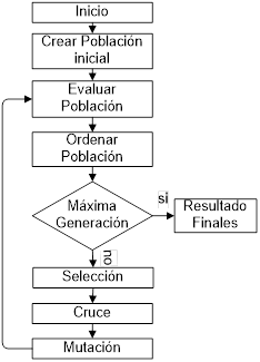
Figura 1. Estructura
del algoritmo genético.
Fuente: elaboración propia.
Población
La población genética está constituida por un
número de cromosomas, en donde cada uno contiene un número de genes. Por la
naturaleza del problema, se definió que cada cromosoma estuviera constituido
por tres genes o variables de números reales, lo cual matemáticamente significa
que un cromosoma es un vector de tres elementos, en donde cada elemento son las
variables proporcional (KP), integral (Ki) y derivativa (Kd). De esta manera,
cada vector (cromosoma) es una probable solución del problema, por lo que la
población genética se ha construido como un arreglo de N filas por tres
columnas, donde N es el número de cromosomas o tamaño de la población y cada
una de las tres columnas representan respectivamente a las variables Kp, Ki y
Kd. La población inicial ha sido creada con números reales aleatorios
respetando los intervalos mínimo y máximo (rangos) de cada variable indicadas
por el usuario. La figura 2 muestra parte del código que crea a la población
genética:
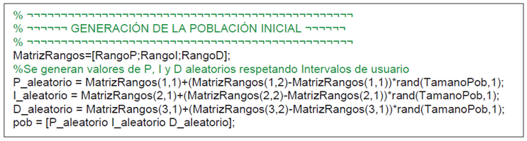
Figura 2. Parte del código que genera la
población genética.
Fuente: elaboración propia.
Selección
En el tipo de selección de ranking lineal, los
cromosomas son clasificados de acuerdo con su valor de ajuste y un rango ri ∈ {1, ..., N} se
asigna a cada uno, donde N es el tamaño de la población. El mejor cromosoma
obtiene el rango N mientras que el peor obtiene el rango 1. Luego: Pi =
(2ri)/N(N+1) es la probabilidad de elegir el i-enésimo cromosoma en el ranking lineal (Pezzella et al.,
2008).
En este sentido, se escogen a los n primeros
cromosomas para cruzarse, donde n es el producto de la tasa de cruce
por el número total de la población. Luego, se le otorga mayor
probabilidad de cruce a los mejores ranqueados, formando un arreglo denominado
«ánfora», en donde los números que identifican a los cromosomas se repiten
proporcionalmente a su importancia (Tejada, 2017). Así, por ejemplo, suponiendo
que se ha escogido a los cuatro primeros cromosomas de la población (1,2,3,4),
con ellos se genera una «ánfora», dando mayor prioridad de ser elegido al
primer cromosoma porque es el mejor ranqueado de la población; esta se
construye de la siguiente manera:
ánfora = (4 3 3 2 2 2 1 1 1 1)
Esto indica que, al seleccionar
aleatoriamente un cromosoma de la «ánfora», el cromosoma 1 tiene la mayor
probabilidad de ser elegido (4/10=40%), seguido del cromosoma 2 (3/10=30%),
luego el cromosoma 3 (2/10=20%) y, finalmente, el cromosoma 4 (1/10=10%).
Después, se selecciona de la «ánfora», mediante un sorteo, los padres y madres
que se aparearán de acuerdo con el número de cruces especificado por el
usuario. Se forman dos vectores, un vector de «padres» y un vector de «madres»,
así como se representan a continuación:
padres = (1 2 1 2 2 1 1 2)
madres = (2 1 2 4 1 3 3 2)
Hasta aquí, la etapa de selección termina su
tarea. Luego, en la etapa de cruce, se van a cruzar los cromosomas: (1, 2), (2,
1), …, (1, 3), (2, 2). Los mismos padres pueden cruzarse varias veces y siempre
van a generar hijos diferentes. Además, puede ocurrir que, tanto el padre como
la madre, sean los mismos cromosomas, por lo que no es necesario evitarlo, esto
no ha afectado el desempeño del algoritmo. La figura 3 muestra parte del código
de la selección:
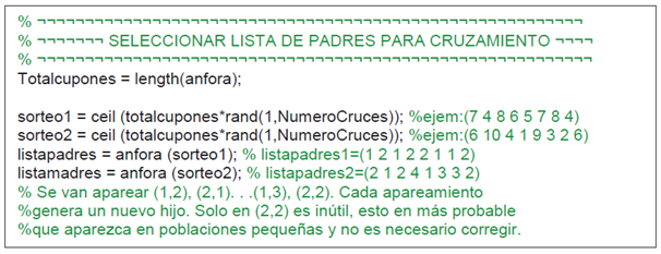
Figura 3. Parte del
código de la selección.
Fuente: elaboración propia.
Cruce
El operador de cruce aritmético de números
reales puede generar hasta dos descendientes que son una combinación lineal de dos
cromosomas X e Y (Yalcinoz y Altun, 2001):
hijo 1 = ![]() X + (1-
X + (1-![]() )Y
)Y
hijo 2 = (1-![]() )X +
)X + ![]() Y
Y
Donde ![]() se escoge aleatoriamente entre 0 y 1.
se escoge aleatoriamente entre 0 y 1.
En esta investigación se ha preferido generar
por cada cruce un solo hijo, por lo que el número de padres es igual al número
de cruces. Esto se ha realizado con el objeto de dar oportunidad a que más
padres generen descendencia obteniendo mayor diversidad en la población. Si se
hubiera optado por generar dos hijos en cada cruce, solo se hubiera
seleccionado para cruzarse la mitad del número de padres. La figura 4 muestra
parte del código de cruce:
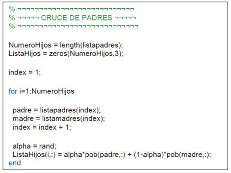
Figura 4. Parte del
código de cruce.
Fuente: elaboración propia.
Mutación
Una vez seleccionado al azar un cromosoma de
la población y la variable que será modificada (Kp, Ki o Kd), esta variable es
remplazada por un número aleatorio:
pob(cromosoma, variable) ß valor aleatorio
Sin embargo, como cada variable tiene un
valor dentro de un intervalo especificado por el usuario (Imin, Imax);
entonces, para evitar que la mutación destruya un valor válido de la variable,
el valor aleatorio tiene que estar dentro de ese rango especificado, por lo que
el reemplazo debe ser (Seck Tuoh, et al.,
2016):
pob(cromosoma, variable) ß Imin + (Imax-Imin)*valor aleatorio
Otro importante punto que se ha tenido en
cuenta es que nunca se elegirá al primer cromosoma para ser mutado, de tal
manera que se conservará sin cambios al mejor rankeado, que pasará a la
siguiente generación. La figura 5 muestra parte del código de mutación:
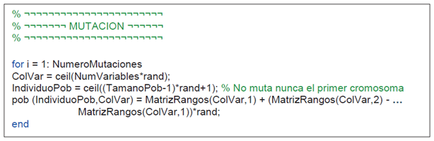
Figura
5. Parte del código de mutación.
Fuente: elaboración propia.
Evaluación
Se ha creado la función PID_ERROR_OBJETIVO,
con la cual se evalúa a cada cromosoma de la población. De esta manera, con los
valores Kp, Ki y Kd de cada cromosoma se calcula la función de transferencia
del controlador PID. Luego, con la función de transferencia del controlador y
con la función de transferencia de la planta del sistema se configura un
sistema cerrado retroalimentado. Finalmente, con el sistema cerrado
retroalimentado se calcula su respuesta frente a la entrada de un escalón de
amplitud uno (1). En todo este proceso, para abreviar cálculos, se han
utilizado las funciones de MATLAB: tf (la cual crea una función de
transferencia de tiempo continuo), series (la que conecta dos modelos o dos
funciones de transferencias) y feedback (encuentra la función de dos modelos,
uno de los cuales pertenece al lazo de realimentación), un procedimiento
similar se realiza en el estudio de Ibrahim Mohamed (2005).
Durante el transitorio que demora la función
de salida hasta alcanzar el valor de 1, se hubiera podido encontrar por cada
cromosoma los valores que toman las siguientes variables: tiempo de subida,
sobreimpulso, tiempo de establecimiento, entre otros. De esta manera, se
hubiera tenido que clasificar a los cromosomas que tengan a esas variables
minimizadas, con lo cual el problema hubiera sido multiobjetivo. Sin embargo,
todas las variables anteriores se pueden correlacionar con una sola variable,
convirtiendo el problema a mono-objetivo. Es por eso que, en este estudio, se
ha optado por calcular por cada cromosoma el error cuadrático medio (ECM) de la
salida.
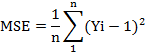
En ese sentido, el progreso del valor de la
salida (Yi) hasta alcanzar el valor del escalón es leído durante n espacios de
tiempo, calculando el error cuadrático medio (ECM) de la siguiente forma:
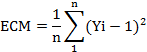
Donde:
n = número de medidas totales
![]() = valor de la salida del sistema en el
instante i
= valor de la salida del sistema en el
instante i
![]() = error cuadrático de la salida
en el instante i con respecto al escalón (1) de entrada.
= error cuadrático de la salida
en el instante i con respecto al escalón (1) de entrada.
Por cada cromosoma de
la población, se tiene que realizar el cálculo de ECM de la manera antes
descrita, con lo cual la función objetivo finaliza su tarea. Posteriormente, el
algoritmo asocia a cada cromosoma un valor de ECM que lo identificará y los
miembros de la población, de acuerdo con su ECM, son ordenados de menor a mayor
valor, garantizando indirectamente un ranking
ordenado de cromosomas de mejores características de tiempo de subida, sobreimpulso
y tiempo de establecimiento. La figura 6 muestra la parte del código de
evaluación:
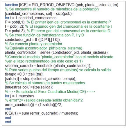
Figura 6. Código de
evaluación.
Fuente: elaboración propia.
El programa de software desarrollado
se ha codificado en el lenguaje de MATLAB. Los resultados, tales como el valor
de Kp, Ki, Kd y las características de la curva de salida, obtenidas con la
función stepinfo, han sido exportados a una hoja de Excel mediante la función
de MATLAB xlswrite, donde también se han generado los gráficos con las curvas de
salida.
Los investigadores que han diseñado sus
propios algoritmos genéticos o algoritmos genéticos difusos, entre otros, han
contrastado sus resultados con los obtenidos con el método clásico de
Ziegler-Nichols, exhibiendo buenos resultados. Por esta razón, se ha creído
conveniente probar el algoritmo diseñado con los modelos de plantas utilizados
por estos investigadores.
RESULTADOS
El programa ha sido ejecutado utilizando los
modelos matemáticos de procesos (plantas) aplicados por otros estudiosos, lo
cual ha permitido comparar resultados. Se ha seleccionado a los autores que han
comparado sus datos con el método clásico de Ziegler-Nichols.
Para todos los casos, el programa se ha
ejecutado con las siguientes especificaciones: tamaño de la población = 40,
número de variables = 3, porcentaje de cruces = 70%, porcentaje de mutación =
10%, número de generaciones = 20.
Las tablas 1-4 muestran el modelo matemático
de la planta controlada, los parámetros del controlador PID (Kp, Ki y Kd), los
valores transitorios de la salida (sobre pico máximo, tiempo de subida, tiempo
de establecimiento) y el error cuadrático medio. Además, se comparan los
resultados con los obtenidos por otros investigadores, la columna «Algoritmo
Genético Propuesto» corresponde al presente trabajo. Los intervalos de búsqueda
para cada variable se muestran en la última fila de cada tabla.
Tabla 1. Comparaciones con resultados para Planta 1.
|
Planta
1
|
Algoritmo
Genético Pareto (Acevedo et al.,
2014) Multivariable |
Algoritmo
Genético PROPUESTO |
|
Kp |
37,6692 |
45,4248 |
|
Ki |
18,9251 |
19,8057 |
|
Kd |
13,0447 |
7,3211 |
|
Sobre
pico máximo (%) |
0,9995 |
1,2674 |
|
Tiempo
de subida (s) |
No
indica |
0,0545 |
|
Tiempo
de establecimiento (s) |
1,14 |
0,0847 |
|
Error
cuadrático medio |
----------------- |
0,0100 |
|
Búsqueda:
0≤kp≥50; 0≤ki≥20; 0≤kd≥20 |
||
Fuente: elaboración propia.
Tabla 2. Comparaciones con resultados para Planta 2.
|
Planta
2
|
Algoritmo
Genético Pareto (Acevedo et al.,
2014) Multivariable |
Algoritmo
Genético PROPUESTO |
|
Kp |
8,4047 |
48,1812 |
|
Ki |
17,1467 |
19,5887 |
|
Kd |
12,0918 |
11,6125 |
|
Sobre
pico máximo (%) |
1,0137 |
1,1786 |
|
Tiempo
de subida (s) |
No
indica |
0,0180 |
|
Tiempo
de establecimiento (s) |
1,9484 |
0,0291 |
|
Error
cuadrático medio |
------------- |
0,0099 |
|
Búsqueda:
0≤kp≥50; 0≤ki≥20; 0≤kd≥20 |
||
Fuente: elaboración propia.
Tabla 3. Comparaciones con resultados para Planta 3.
|
Planta
3. Control de nivel de tres tanques
|
Algoritmo
Genético (Colorado et al., 2018) |
Algoritmo
Genético PROPUESTO |
|
Kp |
0,0361 |
0,03827 |
|
Ki |
0,000731 |
0,00061 |
|
Kd |
0,6999 |
0,63012 |
|
Sobre
pico máximo (%) |
18 |
12,3728 |
|
Tiempo
de subida (seg.) |
10 |
16,3166 |
|
Tiempo
de establecimiento (seg.) |
90 |
86,0968 |
|
Tiempo
de pico |
45 |
33,5201 |
|
Error
cuadrático medio |
---------- |
0,03280 |
|
Búsqueda:
0≤kp≥0.5; 0≤ki≥0.01; 0≤kd≥0.7 |
||
Fuente: Elaboración propia.
Tabla 4. Comparaciones con resultados para Planta 4.
|
Planta
4. Control de nivel de tanque
|
Fuzzy
PD+PID Controller (Souran et al.,
2013) |
Algoritmo
Genético PROPUESTO |
|
Kp |
30 |
39,10042 |
|
Ki |
21,2 |
1,16204 |
|
Kd |
9 |
6,86381 |
|
Sobre
pico máximo (%) |
0,72 |
0 |
|
Tiempo
de subida (seg.) |
No
indica |
0,06548 |
|
Tiempo
de establecimiento (seg.) |
23 |
0,12271 |
|
Error
cuadrático medio |
|
0,01236 |
|
Búsqueda:
0≤kp≥40; 0≤ki≥30; 0≤kd≥20 |
||
Fuente: elaboración propia.
Las figuras 7-10 muestran gráficamente los
resultados de las tablas anteriores, la salida deseada del sistema se muestra
con líneas punteadas y ha sido fijada para una amplitud de 1 (un escalón Step
Response). Además, la línea azul es la salida del sistema que alcanza finalmente
a la salida deseada.
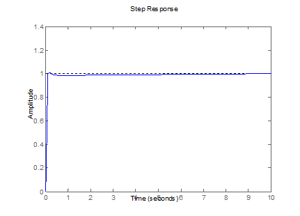
Figura 7.
Respuesta controlada de la Planta 1 (tabla 1).
Fuente: elaboración propia.
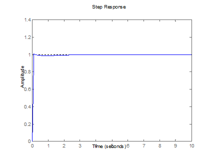
Figura 8. Respuesta
controlada de la Planta 2 (tabla 2).
Fuente: elaboración propia.

Figura 9.
Respuesta controlada de la Planta 3 (tabla 3).
Fuente: elaboración propia.
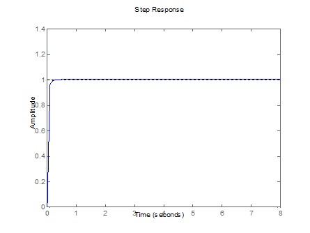
Figura 10.
Respuesta controlada de la Planta 4 (tabla 4).
Fuente: elaboración propia.
.
DISCUSIÓN
Como se puede observar de los resultados de
las tablas 1-4, en todos los casos los sobre picos máximos han sido similares,
los tiempos de establecimientos han sido superiores en todos los casos y solo
en la tabla 3 el tiempo de subida no ha sido el mejor. Estos resultados
demuestran que el algoritmo propuesto ha tenido un buen desempeño en encontrar
los valores adecuados de Kp, Ki y Kd del controlador PID. Además, para todos
los casos se ha utilizado las mismas especificaciones de tamaño de población,
porcentaje de cruce, porcentaje de mutación y número de generaciones lo cual
demuestra que el algoritmo es bastante robusto.
CONCLUSIONES
Mediante algoritmos genéticos, se ha
solucionado el problema de sintonizar los parámetros proporcional, derivativo e
integral de un controlador PID, minimizando el tiempo de establecimiento y el
sobreimpulso de la respuesta en plantas no lineales. Asimismo, se ha probado
que los resultados obtenidos han sido óptimos al compararlos con resultados de
otras investigaciones, mostrados en las tablas 1-4.
Además, se ha probado que el algoritmo
diseñado como mono-objetivo ha sido eficiente al minimizar, indirectamente,
diversas variables (sobreimpulso, tiempo de establecimiento, tiempo de subida)
mediante la minimización de una sola variable: el
error cuadrático medio, en contraposición con un algoritmo genético
multiobjetivo basado en el enfoque de Pareto, como el presentado por Acevedo et al.
(2014).
REFERENCIAS BIBLIOGRÁFICAS
[1]
Acevedo, B.; Fonseca, J. y Gómez, J. (2014). Desarrollo
de una herramienta en Matlab para sintonización de controladores PID,
utilizando algoritmos genéticos basado en técnicas de optimización
multiobjetivo. Revista SENNOVA, 1(1), 80-103.
[2]
Akbari-Hasanjani, R.; Javadi, S. y Sabbaghi-Nadooshan, R.
(2015). DC motor speed control by self-turning fuzzy PID
algorithm. Transactions of the Institute of Measurement and Control, 37(2),
164-176.
[3]
Beck, F. (2000). Escalonamiento de tarefas job-shop
realistas utilizando algoritmos genéticos en Matlab. (Tesis de maestría).
Universidad Federal de Santa Catarina, Florianópolis, SC.
[4]
Colorado, O.; Hernández, N.; Seck Tuoh, J. y Medina, J. (2018).
Algoritmo genético aplicado a la sintonización de un controlador PID para un
sistema acoplado de tanques. PADI Boletín Científico de Ciencias Básicas e
Ingenierías del ICBI, 5(10), 50-55.
[5]
Feng, H.; Yin, C.;
Weng, W.; Ma, W.; Zhou, J.; Jia, W. y Zhang, Z. (2018). Robotic excavator
trajectory control using an improved GA based PID controller. Mechanical Systems
and Signal Processing, 105, 153-168.
[6]
Gestal, M.; Rivero, D.; Rabuñal, J.; Dorado, J. y Pazos,
A. (2010). Introducción a los algoritmos genéticos y la programación
genética. La Coruña, España: Universidad de La Coruña.
[7]
Haupt, R. y Haupt, S. (2004). Practical genetic
algorithms. Nueva Jersey, EE. UU.: Wiley-Interscience.
[8]
Hernández, R.; García, L.; Salgado, T.; Gómez, A. y
Fonseca, F. (2016). Neural network-based self-turning
PID control for underwater vehicles. Sensors, 16(9). Recuperado de https://www.ncbi.nlm.nih.gov/pmc/articles/PMC5038707/.
[9]
Iwan, M.; Fook, L. y
Leap, M. (2011). Tuning of PID controller using particle swarm optimization
(PSO). International Journal on Advanced Science, Engineering and
Information Technology, 1(4), 458-461. Recuperado de http://insightsociety.org/ojaseit/index.php/ijaseit/article/viewFile/93/98.
[10] Lahlouh, I.;
Elakkary, A. y Sefiani, N. (2019). PID controller
of a MIMO system using ant colony algorithm and its application to a poultry
house system. En H. Hachimi (Ed.), 2019 5th International Conference on
Optimization and Application (ICOA) llevado a cabo en Marruecos.
[11] Mohamed, I. (2005). The PID controller design using genetic algorithm.
(Tesis de pregrado). University of Southern Queensland, Toowoomba, QLD.
[12] Pezzella, F.; Morganti,
G. y Ciaschetti, G. (2008). A genetic algorithm
for the flexible job-shop scheduling problema. Computers &
Operations Research, 35(10), 3202-3212.
[13] Schaffer, J. y Eshelman, L. (1991). On crossover as an evolutionarily
viable strategy. International Conference on Genetic Algorithms, 4, 61-68.
[14] Seck Tuoh, J.;
Medina, J. y Hernández, N. (2016). Introducción a los algoritmos genéticos
con Matlab. Recuperado de
https://repository.uaeh.edu.mx/bitstream/bitstream/handle/123456789/16991/introduccion_a_los_algoritmos_geneticos_con_matlab.pdf.
[15] Souran, D.; Abbasi, S. y Shabaninia, F. (2013). Comparative study
between tank’s water level control using PID and fuzzy logic controller. En V.
Balas, J. Fodor, A. Várkonyi-Kóczy, J. Dombi y L. Jain (Eds.), Soft
computing applications V. 195 (pp. 141-153). Berlín, Alemania:
Springer-Verlag Berlin Heidelberg.
[16] Srinivas, M. y Patnaik, L. (1994). Adaptive probabilities of crossover and mutation in genetic algorithms. IEEE
Transactions on Systems, Man, and Cybernetics, 24(4), 656-667.
[17] Tejada, G. (2017). Enrutamiento
y secuenciación óptimos en un flexible job shop multiobjetivo mediante
algoritmos genéticos. (Tesis
doctoral). Universidad Nacional Mayor de San Marcos, Lima.
[18] Yalcinoz, T. y Altun,
H. (2001). Power economic dispatch using a
hybrid genetic algorithm. IEEE Power Engineering Review, 21(3),
59-60.
Revista Industrial Data 22(2): 213-234 (2019) Guillermo Tejada
DOI: http://dx.doi.org/10.15381/idata.v22i2.16489
ISSN: 1560-9146 (Impreso) / ISSN:
1810-999
Received: 21/07/2019
Accepted: 23/09/2019
PID CONTROLLER WITH REAL NUMBER GENETIC ALGORITHMS
Guillermo
Tejada Muñoz[2]
ABSTRACT
A genetic
algorithm (GA) is an artificial intelligence technique that can be applied to
any engineering specialty. In this study, the proposed GA finds optimal values
for PID controller parameters Kp, Ki and Kd, which are widely used in the
industry. Chromosomes, composed of Kp, Ki and Kd genes, represented by real
numbers, evolve and are evaluated by the mean square error (MSE) of the desired
output. In that sense, the solution is the chromosome with the lowest MSE,
which produces less transient output. In addition, the GA has been encoded in
MATLAB language and results have been compared with other works.
Keywords:
genetic algorithms, real number genes, PID, mean square error.
INTRODUCTION
An industrial
process can be considered a closed-loop (feedback) system consisting of a
controller and a controlled plant. For controller
design, one of the most used techniques, due to its simplicity and robustness,
is the so-called proportional integral derivative (PID); however, it is not an
easy task to find the optimal values of controller parameters Kp, Ki and Kd.
For this reason, artificial intelligence algorithms have been proposed as a
solution for the calculation of these parameters, for example: particle swarm
optimization (PSO) (Iwan et al.,
2011), ant colony optimization (ACO) (Lahlouh et al., 2019), fuzzy logic (Akbari-Hasanjani et al., 2015), neural networks (Hernández et al., 2016) and genetic algorithms (GA) (Feng et al., 2018) among others. This study
describes the development of a GA, encoded in MATLAB’s M-language, that
calculates the controller’s Kp, Ki and Kd parameters, so that the output of the
system (controller plus plant) reaches the desired value, minimizing transient
overshoot values, settling time and rise time.
A genetic algorithm (GA) is a search algorithm
that follows the evolutionary paradigm. From an initial population, the
algorithm applies genetic operators (selection, crossover and mutation) to
produce offspring (in local search terminology, neighborhood search method),
who are clearly fitter than their parents. In each generation (iteration), each
new chromosome corresponds to a solution (Pezzella et al., 2008). The
methods for selecting the chromosomes that will generate descendants prioritize
those with higher fitness values; among these selection methods are the
following: roulette wheel selection, tournament selection, linear ranking, etc.
In this study, linear ranking selection was used because it makes it possible
to assign the chromosomes, ranked according to their fitness value, probability
values that differentiated in a decreasing linear proportion the best
to the worst ranked; that is to say, the probabilities the chromosomes have of
being selected are not differentiated disproportionately.
The
methods for crossing chromosomes are diverse and depend on the nature of the
genes, which can be binary, permutation, real-number, etc. Among crossing
methods are the following: single point exchange (SPX), double point crossover
(DPX), partially matched crossover (PMX), order crossover (OX), cycle crossover
(CX), arithmetic crossover, etc. (Haupt & Haupt, 2004). This last one, the
arithmetic crossover, has been used in this study, because it is suitable for
real-number genes. Thus, while crossing tends to converge the genetic
population, preferably at optimal values, mutation aims to maintain a certain
level of diversity within the population, that is, to prevent the population
from converging rapidly (Srinivas & Patnaik, 1994; Schaffer & Eshelman,
1991; Beck, 2000). The most frequently used mutation is one in which one of the
chromosome genes (variables) randomly varies (Gestal et al., 2010). Lastly, the number of mutations is calculated as a
percentage of population size.
Therefore, the problem to be solved is multi-objective, because the idea is
to minimize more than one variable, which
are: overshoot, settling time and rise time of the system response. However,
for simplicity’s sake, the problem has been treated as a mono-objective, that
is, pursuing a single objective, which is correlated with the variables of
interest. In this sense, the mean square error (MSE) of the output has been
selected as the objective function, also called the fitness function,
evaluation function or cost function.
On the other hand, the program code was written in MATLAB language. The
program was run monitoring the plants used by other
researchers. In this way it was possible to compare results and demonstrate
that the proposed algorithm performed well, since it found the appropriate PID
controller Kp, Ki and Kd values, which have minimized overshoot, settling time
and rise time of the system response.
METHODOLOGY
The structure of the implemented algorithm is described in Figure 1.
After creating an initial genetic population, each chromosome in the population
is evaluated by calculating the mean square error (MSE) of the corresponding output.
Next, the chromosomes are ordered from the lowest to the highest value
according to their MSE and, subsequently, the most suitable chromosomes are
selected to be crossed in order to generate offspring, randomly mutating the
chromosomes for further evaluation. The process is repeated as many times as
the number of generations indicated by the user permits. Finally, the optimal
population will be obtained and the best chromosome will be at the top of the
list. Further details on each stage are provided in the following paragraphs.
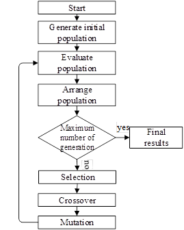
Figure 1. Genetic algorithm structure.
Source: Prepared by the author.
Population
The genetic population consists of a number of chromosomes, each
containing a number of genes. Due to the nature of the problem, each chromosome
was made up of three real-number genes or variables, which mathematically means
that a chromosome is a vector of three elements, which are Kp (proportional),
Ki (integral) and Kd (derivative) variables. Consequently, each vector
(chromosome) is a likely solution to the problem, therefore the genetic
population was built as an arrangement of N rows with three columns, where N is
the number of chromosomes or population size and each of the three columns
represent the variables Kp, Ki and Kd, respectively. The initial population was
created with random real numbers respecting the minimum and maximum intervals
(ranges) of each variable indicated by the user. Figure 2 shows a portion of
the code that creates the genetic population:
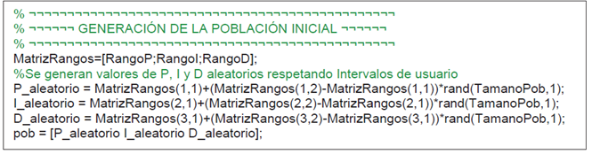
Figure 2. Portion of the code that generates the genetic population.
Source: Prepared by the author.
Selection
In linear
ranking selection, chromosomes are classified according to their fitness value
and a range ri ∈ {1, ..., N} is assigned to each of
them, where N is the size of the population. The best chromosome obtains range
N while the worst gets range 1. Then: Pi = (2ri)/N(N+1) is the probability of
choosing the i-nth chromosome in the linear ranking (Pezzella et al., 2008).
In this
sense, the first n chromosomes are selected for crossover, where n is the
product of the rate of crossing by the total population number. Then, greater
probability of crossing is given to the best ranked, forming an arrangement
referred to as “strand”, where the numbers that identify the chromosomes are
repeated proportionally to their importance (Tejada, 2017). For example, assuming
that the first four chromosomes in the population have been chosen (1,2,3,4),
they generate a “strand”, giving the first chromosome higher priority because
it is the best ranked within the population. It is constructed as follows:
strand = (4 3
3 2 2 2 1 1 1 1)
This
indicates that, by randomly selecting a chromosome from the “strand”,
chromosome 1 is most likely to be chosen (4/10=40%), followed by chromosome 2
(3/10=30%), then chromosome 3 (2/10=20%) and finally chromosome 4 (1/10 = 10%).
Next, from the “strand”, the parents who will be mated according to the number
of crossovers specified by the user, are randomly selected. Two vectors are
formed, a “father” vector and a “mother” vector, as follows:
fathers = (1
2 1 2 2 1 1 2)
mothers = (2
1 2 4 1 3 3 2)
At this
point, selection ends. Next, crossover begins, and the chromosomes to be
crossed are: (1, 2), (2, 1), …, (1, 3), (2, 2). The same parents can crossover
several times and will always generate different
offspring (children). In addition, it may happen that both the father and the
mother are the same chromosomes; it is not necessary to avoid this, as it has
not affected the performance of the algorithm. Figure 3 shows a portion of the
selection code:
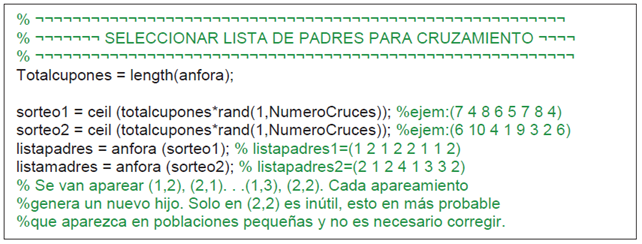
Figure 3. Portion of the selection code.
Source: Prepared by the author.
Crossover
An arithmetic crossover operator of real numbers may produce up to two
offspring, which are a linear combination of two chromosomes X and Y (Yalcinoz
& Altun, 2001):
child 1
= ![]() X + (1-
X + (1-![]() )Y
)Y
child 2
= (1-![]() )X +
)X + ![]() Y
Y
where ![]() is a random number between 0 and
1.
is a random number between 0 and
1.
In this study the preference was to generate one child per crossover, so
the number of parents is equal to the number of
crossovers. This has been done in order to give more parents the opportunity to
generate offspring, obtaining greater diversity in the population. If it had
been decided to produce two children at each crossover, only half of the number
of parents would have been selected for crossover. Figure 4 shows a portion of the crossover code:
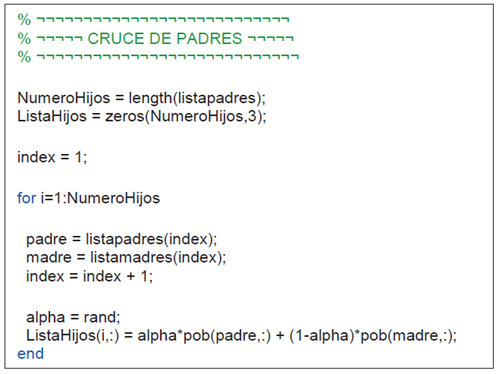
Figure 4. Portion of the crossover code.
Source: Prepared by the author.
Mutation
Once a chromosome and variable to be modified (Kp, Ki or Kd) have been
randomly selected from the population, as well as the variable to be modified
(Kp, Ki or Kd), the variable is replaced by a random number:
pop(chromosome, variable) ß random value
However, since each variable has a value within a user-specified range
(minI, maxI), the random value has to be within that specified range in order
to prevent mutation from destroying a valid value of the variable, thus the
replacement must be (Seck Tuoh, et al.,
2016):
pop(chromosome, variable) ß minI + (maxI-minI)*random value
Another important point that has been taken into account is that the
first chromosome will never mutated so that the highest ranked chromosome,
which will pass to the next generation, will remain unchanged. Figure 5 shows a
portion of the mutation code:
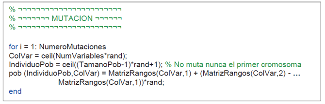
Figure 5. Portion of the mutation
code.
Source: Prepared by the author.
Evaluation
Function PID_ERROR_OBJETIVO has been created, with which each chromosome
in the population is evaluated. Thus, the transfer function of the PID
controller is calculated using the Kp, Ki and Kd values of
each chromosome. Subsequently, with the controller transfer function and the
system plant transfer function, a close-loop feedback system is configured.
Finally, response to the input of a step of amplitude one (1) is calculated
using the closed-loop system. The following MATLAB functions have been used to abbreviate calculations throughout the entire process:
tf (which creates a continuous-time transfer function), series (which connects
two models or two transfer functions) and feedback (finds the function of two
models, one of which belongs to the feedback loop). A similar procedure is
performed in the study by Ibrahim Mohamed (2005).
During the
transient response time it takes the output function to reach a value of 1, it
would have been possible to find the values taken by the following variables,
per chromosome, could have been found: rise time, overshoot, settling time,
among others. Accordingly, chromosomes with minimized variables would have had
to be classified, and as a result, the problem would have been multi-objective.
However, all the above variables can be correlated with a single variable,
producing a single-objective problem. For that reason, in this study, it was
decided to calculate the mean square error (MSE) of the output per chromosome.
In this sense, the progress of the output value (Yi) until reaching the
step value is read over n intervals of time, calculating the mean square error
(MSE) as follows:
Where:
n = total
number of intervals
![]() = system output
value at moment i
= system output
value at moment i
![]() = mean square error of the output at moment i
regarding input step (1)
= mean square error of the output at moment i
regarding input step (1)
For each chromosome in the population, the MSE calculation has to be
performed as described above, and thus the objective function completes its
task. Subsequently, the algorithm associates a MSE value to each chromosome,
which will identify it; the members of the population are ordered from lowest
to highest value according to their MSE, indirectly guaranteeing an orderly
ranking of chromosomes with better characteristics of rise time, overshoot and
settling time. Figure 6 shows a portion of the evaluation code:
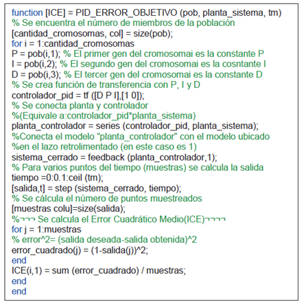
Figure 6. Evaluation code.
Source: Prepared by the author.
The software developed has been encoded in
MATLAB language. The results, such as Kp, Ki, Kd values and the output curve’s characteristics
obtained by means of stepinfo function, have been exported to an Excel sheet
using the MATLAB xlswrite function, where output curves plots have also been
generated.
Researchers
who have designed their own genetic algorithms or fuzzy genetic algorithms,
among others, have contrasted their results with those obtained with the
classic Ziegler-Nichols method, obtaining good results. For this reason, it was
considered appropriate to test the algorithm designed with the plant models
used by these researchers.
RESULTS
The program
has been executed using the mathematical models of processes (plants) applied
by other scholars, which allowed us to compare results. Authors who have
compared their data against the classic Ziegler-Nichols method have been
selected.
For all cases, the program has been executed considering the following
specifications: population size = 40, number of variables = 3, percentage of
crossover = 70%, percentage of mutation = 10%, number of generations
= 20.
Tables 1-4
show the mathematical model of the controlled plant, the PID controller’s
parameters (Kp, Ki and Kd), the output transient values (maximum overshoot,
rise time, settling time) and the mean square error. In addition, the results are compared with those obtained by other researchers, and the column
“Proposed genetic algorithm” corresponds to this study. The search intervals
for each variable are displayed in the last row of each table.
Table 1. Comparison against
results for Plant 1.
|
Plant 1
|
Pareto multi-objective genetic algorithm (Acevedo et al., 2014) |
Proposed genetic
algorithm |
|
Kp |
37.6692 |
45.4248 |
|
Ki |
18.9251 |
19.8057 |
|
Kd |
13.0447 |
7.3211 |
|
Maximum overshoot
(%) |
0.9995 |
1.2674 |
|
Rise time (s) |
Not indicated |
0.0545 |
|
Settling time (s) |
1.14 |
0.0847 |
|
Mean square error |
----------------- |
0.0100 |
|
Search: 0≤kp≥50;
0≤ki≥20; 0≤kd≥20 |
||
Source: Prepared by the author.
Table 2. Comparison against
results for Plant 2.
|
Plant 2
|
Pareto multi-objective genetic algorithm (Acevedo et al.,
2014) |
Proposed genetic
algorithm |
|
Kp |
8.4047 |
48.1812 |
|
Ki |
17.1467 |
19.5887 |
|
Kd |
12.0918 |
11.6125 |
|
Maximum overshoot
(%) |
1.0137 |
1.1786 |
|
Rise time (s) |
Not indicated |
0.0180 |
|
Settling time (s) |
1.9484 |
0.0291 |
|
Mean square error |
------------- |
0.0099 |
|
Search: 0≤kp≥50;
0≤ki≥20; 0≤kd≥20 |
||
Source: Prepared by the author.
Table 3. Comparison against
results for Plant 3.
|
Plant 3. Control of
three tanks’ level
|
Genetic algorithm (Colorado et al.,
2018) |
Proposed genetic
algorithm |
|
Kp |
0.0361 |
0.03827 |
|
Ki |
0.000731 |
0.00061 |
|
Kd |
0.6999 |
0.63012 |
|
Maximum overshoot
(%) |
18 |
12.3728 |
|
Rise time (sec.) |
10 |
16.3166 |
|
Settling time
(sec.) |
90 |
86.0968 |
|
Peak time |
45 |
33.5201 |
|
Mean square error |
---------- |
0.03280 |
|
Search: 0≤kp≥0.5; 0≤ki≥0.01; 0≤kd≥0.7 |
||
Source: Prepared by the author.
Table 4. Comparison against
results for Plant 4.
|
Plant 4. Control of
tank level
|
Fuzzy PD+PID
Controller (Souran et al., 2013) |
Proposed genetic
algorithm |
|
Kp |
30 |
39.10042 |
|
Ki |
21.2 |
1.16204 |
|
Kd |
9 |
6.86381 |
|
Maximum overshoot
(%) |
0.72 |
0 |
|
Rise time (sec.) |
Not indicated |
0.06548 |
|
Settling time
(sec.) |
23 |
0.12271 |
|
Mean square error |
|
0.01236 |
|
Search: 0≤kp≥40;
0≤ki≥30; 0≤kd≥20 |
||
Source: Prepared by the author.
Figures 7-10 graphically show the results of the above tables. The
desired output of the system is shown with dotted lines and has been set to an
amplitude of 1 (one step response). In addition, the blue line is the
system output that finally reaches the desired output.

Figure 7. Controlled response from Plant 1 (Table 1).
Source: Prepared by the author.

Figure 8. Controlled response from Plant 2 (Table 2).
Source: Prepared by the author.
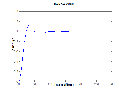
Figure 9. Controlled response from Plant 3 (Table 3).
Source: Prepared by the author.

Figure 10. Controlled response from Plant 4 (Table 4).
Source: Prepared by the author.
DISCUSSION
As can be seen from the results in Tables 1-4, in all cases maximum
overshoot values were similar. Settling times were superior in all cases and
rise time was best in all but Table 3. These results show that the proposed
algorithm performed well in finding the appropriate Kp, Ki and Kd values for
the PID controller. In addition, the same specifications of population size,
crossover percentage, mutation percentage and number of generations were used
for all cases, demonstrating that the algorithm is quite robust.
CONCLUSIONS
Using genetic algorithms, the problem of tuning the proportional,
derivative and integral parameters of a PID controller was solved, minimizing
settling time and overshoot of the response in non-linear plants. It was also
demonstrated that the results obtained were optimal when compared with the
results of other investigations, shown in Tables 1-4.
In addition, it was demonstrated that the algorithm designed as a
single-objective is efficient by indirectly minimizing various variables
(overshoot, settling time, rise time) by minimizing a single variable: mean square error, as opposed to a multi-objective
genetic algorithm based on the Pareto approach, as presented by Acevedo et al. (2014).
REFERENCES
[1]
Acevedo, B.; Fonseca, J. & Gómez, J. (2014).
Desarrollo de una herramienta en Matlab para sintonización de controladores
PID, utilizando algoritmos genéticos basado en técnicas de optimización
multiobjetivo. Revista SENNOVA, 1(1), 80-103.
[2]
Akbari-Hasanjani, R.; Javadi, S. &
Sabbaghi-Nadooshan, R. (2015). DC motor speed
control by self-turning fuzzy PID algorithm. Transactions of the Institute of
Measurement and Control, 37(2), 164-176.
[3]
Beck, F. (2000). Escalonamiento de tarefas job-shop
realistas utilizando algoritmos genéticos en Matlab. (Master’s thesis).
Universidad Federal de Santa Catarina, Florianópolis, SC.
[4]
Colorado, O.; Hernández, N.; Seck Tuoh, J. & Medina,
J. (2018). Algoritmo genético aplicado a la sintonización de un controlador PID
para un sistema acoplado de tanques. PADI Boletín Científico de Ciencias
Básicas e Ingenierías del ICBI, 5(10), 50-55.
[5]
Feng, H.; Yin, C.;
Weng, W.; Ma, W.; Zhou, J.; Jia, W. & Zhang, Z. (2018). Robotic excavator
trajectory control using an improved GA based PID controller. Mechanical Systems
and Signal Processing, 105, 153-168.
[6]
Gestal, M.; Rivero, D.; Rabuñal, J.; Dorado, J. &
Pazos, A. (2010). Introducción a los algoritmos genéticos y la programación
genética. La Coruña, Spain: Universidad de La Coruña.
[7]
Haupt, R. &
Haupt, S. (2004). Practical genetic algorithms. New Jersey, USA: Wiley-Interscience.
[8]
Hernández, R.; García, L.; Salgado, T.; Gómez, A. &
Fonseca, F. (2016). Neural network-based self-turning
PID control for underwater vehicles. Sensors,
16(9). Retrieved from https://www.ncbi.nlm.nih.gov/pmc/articles/PMC5038707/.
[9]
Iwan, M.; Fook, L.
& Leap, M. (2011). Tuning of PID controller using particle swarm optimization
(PSO). International Journal on Advanced Science, Engineering and
Information Technology, 1(4), 458-461. Retrieved from
http://insightsociety.org/ojaseit/index.php/ijaseit/article/viewFile/93/98.
[10]
Lahlouh, I.;
Elakkary, A. & Sefiani, N. (2019). PID controller of a MIMO system using
ant colony algorithm and its application to a poultry house system. In H.
Hachimi (Ed.), 2019 5th International Conference on Optimization and
Application (ICOA) llevado a cabo en Marruecos.
[11]
Mohamed, I. (2005). The
PID controller design using genetic algorithm. (Bachelor thesis).
University of Southern Queensland, Toowoomba, QLD.
[12]
Pezzella, F.; Morganti, G. & Ciaschetti, G. (2008). A genetic algorithm for the flexible job-shop scheduling problema. Computers
& Operations Research, 35(10), 3202-3212.
[13]
Schaffer, J. &
Eshelman, L. (1991). On crossover as an evolutionarily viable strategy. International
Conference on Genetic Algorithms, 4, 61-68.
[14]
Seck Tuoh, J.; Medina, J. & Hernández, N. (2016). Introducción
a los algoritmos genéticos con Matlab. Retrieved from
https://repository.uaeh.edu.mx/bitstream/bitstream/handle/123456789/16991/introduccion_a_los_algoritmos_geneticos_con_matlab.pdf.
[15]
Souran, D.; Abbasi,
S. & Shabaninia, F. (2013). Comparative study between tank’s water level
control using PID and fuzzy logic controller. In V. Balas, J. Fodor, A.
Várkonyi-Kóczy, J. Dombi y L. Jain (Eds.), Soft computing applications V.
195 (pp. 141-153). Berlin, Germany: Springer-Verlag Berlin Heidelberg.
[16]
Srinivas, M. &
Patnaik, L. (1994). Adaptive probabilities of crossover and mutation in genetic
algorithms. IEEE Transactions on Systems, Man, and Cybernetics, 24(4),
656-667.
[17]
Tejada, G. (2017). Enrutamiento y secuenciación
óptimos en un flexible job shop multiobjetivo mediante algoritmos genéticos. (PhD thesis). Universidad
Nacional Mayor de San Marcos, Lima.
[18] Yalcinoz, T. & Altun, H. (2001). Power economic dispatch using a hybrid genetic algorithm. IEEE Power Engineering Review, 21(3), 59-60.