Revista Industrial Data 24(1): 243-276 (2021)
DOI: https://dx.doi.org/10.15381/idata.v24i1.18930
ISSN: 1560-9146 (Impreso) / ISSN: 1810-9993 (Electrónico)
Recibido: 22/10/2020
Aceptado: 07/12/2020
Publicado: 26/07/2021
Modelación del promedio mensual de los valores cuota por AFP y fondo tipo 2 con la metodología Box y Jenkins o ARIMA
Wilfredo Bazán Ramírez[1]
RESUMEN
Las crisis económicas y financieras en el mundo son recurrentes por la presentación de diversos patrones. Estas crisis han afectado las rentabilidades del sistema privado de pensiones del Perú, sin respuestas efectivas por parte de las Administradoras de Fondos de Pensiones (AFP). Con la metodología Box y Jenkins o modelo autorregresivo integrado de promedio móvil (ARIMA) se describe y pronostica, por cada AFP, el comportamiento de las rentabilidades del promedio mensual de los valores cuota diarios del fondo tipo 2, que inició en diciembre del 2005. Las inversiones de este fondo están distribuidas en 55% en renta fija y 45% en renta variable, con un perfil balanceado destinado a trabajadores entre 45 a 60 años. El tipo de dato de las rentabilidades del promedio mensual del fondo tipo 2 corresponde a series de tiempo estacionarias en sentido débil, pues los primeros momentos como la media, y la varianza y la autocovarianza son invariantes en el tiempo.
Palabras clave: series de tiempo, rentabilidad, estacionariedad en sentido débil, raíz unitaria, ruido blanco.
INTRODUCCIÓN
Con la metodología Box y Jenkins o autorregresivo integrado de promedio móvil (ARIMA, por sus siglas en inglés) se describió y pronosticó el comportamiento de las rentabilidades del promedio mensual de los valores diarios del fondo tipo 2, que inició en diciembre del 2005, de cada Administradora de Fondo de Pensiones (AFP). El tipo de dato de las rentabilidades mensuales del fondo tipo 2 corresponde a las series de tiempo y, para que puedan modelarse con ARIMA, necesariamente deben ser estacionarias en sentido débil, donde los dos primeros momentos como la media, y la varianza y la autocovarianza deben ser invariantes en el tiempo.
En 1976, Box y Jenkins formalizaron la metodología Box-Jenkins y los modelos ARIMA, también conocidos como modelos Box-Jenkins, donde se refieren a las series de tiempo que se sustentan en los procesos estocásticos (Box, Jenkins y Reinsel, 2008). Cuando se pronostica con un modelo ARIMA, se siguen los siguientes pasos:
1. Identificación
2. Estimación
3. Validación
4. Pronóstico
Estos pasos se grafican en Box et al. (2008), donde se les denomina “Etapas en el enfoque iterativo de la construcción de modelos” (p.18).
Gujarati y Porter (2010) sostienen que cuando una serie de tiempo no es estacionaria, la media y la varianza no son invariantes en el tiempo. Asimismo, al referirse a la metodología Box y Jenkins ARIMA, agregan lo siguiente:
La publicación de G. P. E. Box y G. M. Jenkins Time Series Analysis: Forecasting and Control, op. cit., marcó el comienzo de una nueva generación de herramientas de pronóstico. Popularmente conocida como metodología de Box-Jenkins (BJ), pero técnicamente conocida como metodología ARIMA, el interés de estos métodos de pronósticos no está en la construcción de modelos uniecuacionales o de ecuaciones simultáneas, sino en el análisis de las propiedades probabilísticas, o estocásticas, de las series de tiempo económicas por sí mismas (…). A diferencia de los modelos de regresión, en los cuales Yt se explica por las k regresoras X1, X2, X3, ..., Xk, en los modelos de series de tiempo del tipo BJ, Yt se explica por valores pasados o rezagados de sí misma y por los términos de error estocásticos. Por esta razón, los modelos ARIMA reciben algunas veces el nombre de modelos ateóricos —porque no se derivan de teoría económica alguna—. (pp. 774-775)
Court y Rengifo (2011) señalan que “El concepto de estacionariedad tiene dos versiones: la estacionariedad estricta y la estacionariedad débil” (p. 400); a continuación, se muestran cada una de estas:
Estacionariedad estricta. Es un proceso estocástico {yi} con i = 1, 2, …, T. Es estrictamente estacionario si, para un número real finito R y para cualquier conjunto de subíndices i1, i2, …, iT, se define de esta forma:

Estacionariedad débil. Es un proceso estocástico {yi} con i = 1, 2, …, T. Es débilmente estacionario si se cumple lo siguiente:

Ramón y López (2016) también identifican dos tipos de estacionariedad: en sentido fuerte y en sentido débil. Para el primer caso, los cuatro momentos de las distribuciones conjuntas son invariantes en el tiempo, y para el segundo, solo los 2 primeros momentos lo son. En este caso la metodología Box y Jenkins se basa en la estacionariedad en sentido débil.
Situación problemática
Ñaupas et al. (2014) indican que en la vida cotidiana se presentan patrones repetitivos, pero con ciertas características diferentes, y agregan que la predicción de los fenómenos naturales es más certera que los fenómenos sociales:
Así por ejemplo, conociendo las leyes de Kepler, que explican los movimientos de traslación de los planetas, satélites, cometas y asteroides es posible calcular la ocurrencia de eclipses, mareas y acercamiento de cometas a la órbita de la Tierra. La predicción del tiempo, de inundaciones, terremotos, huracanas, erupciones volcánicas, la ocurrencia de mareas, o de pandemias son más confiables que las ocurrencias de revoluciones, conflictos sociales, golpes de estado, etc. (apartado 2.4.2. ¿Qué es la investigación natural?)
Estos fenómenos, que originan crisis, impactan negativamente en las economías y las finanzas, por lo cual Mira (2016) plantea la aparición recurrente de crisis financieras. Estas crisis han afectado reiteradamente las rentabilidades del sistema privado de pensiones en el Perú.
La Organización Internacional del Trabajo (OIT) estableció en 1933 el convenio sobre el seguro de vejez, y en 1952 determinó los lineamientos sobre las prestaciones de vejez. En el Perú inicialmente funcionaba el Sistema Nacional de Pensiones (SNP), que actualmente es administrado por la Oficina de Normalización Previsional (ONP). Entre 1981 y 2014, tal como señalan Ortiz, Durán-Valverde, Urban, Wodsak y Yu (2019), unos 30 países privatizaron total o parcialmente sus pensiones públicas obligatorias, hecho que sucedió en el Perú en el año 1993. La Asociación de Administradoras de Fondo de Pensiones (2018) define la pensión en el sistema privado de pensiones peruano (SPP) como “el ingreso periódico que recibe el afiliado como consecuencia de un proceso previo de suavización de consumo, a través del ahorro a lo largo de su vida laboral en su cuenta de capitalización individual (CIC)” (p. 8), con la finalidad de que el trabajador ya jubilado no tenga dificultades económicas.
Las administradoras de fondos de pensiones (AFP) se encargan de administrar los aportes de cada individuo durante su vida laboral, es decir, invierten sus ahorros a fin de obtener rentabilidad para que este, una vez jubilado, pueda disfrutar de sus aportes y sus ganancias sin necesidad de depender de sus familiares o del Estado. Sin embargo, Cruz-Saco et al. (2014) advirtieron que el sistema previsional en el Perú era “ineficiente, tiene una baja probabilidad de incrementar apreciablemente la cobertura en los siguientes 36 años, y presenta, además, un conjunto de inequidades en la asignación de los beneficios previsionales” (p. 2).
Flórez (2014) también agrega que “los ahorros para la jubilación de millones de personas se encuentran expuestos, de manera intrínseca, al comportamiento favorable, así como adverso, de los mercados financieros” (p. 121). Estas situaciones generan una alta volatilidad, sobre todo cuando se presentan más noticias negativas con respecto a las noticias positivas, con lo cual se observa un comportamiento asimétrico del mercado, principalmente el de renta variable.
Ortiz et al. (2019) sostienen que “Los trabajadores se convirtieron así en consumidores obligados del sector financiero, con lo que asumían individualmente todos los riesgos del mercado financiero sin contar con la suficiente información para tomar decisiones sensatas” (p. 803). Es decir, cuando el mercado es estable o se presentan buenas noticias, los rendimientos serán positivos. Por su lado, a decir de Yang et al. (como se citó en Gutiérrez et al., 2017), las crisis financieras se han caracterizado por el incremento del riesgo y alta volatilidad, lo que ha afectado negativamente los rendimientos. Es decir, en el caso del SPP se presentaron noticias negativas y, en consecuencia, las altas expectativas que inicialmente generó se fueron diluyendo con el trascurrir de los años debido a que no produjo los resultados esperados.
Carlos Palomino, en una entrevista a RTV San Marcos - UNMSM (2020), indicó que las inversiones de las AFP ingresan a mecanismos bursátiles y no a activos tangibles. Estos instrumentos bursátiles son volátiles debido a los ciclos o choques económicos que, a su vez, son consecuencia de variables externas al sistema, como, por ejemplo, una pandemia.
Cabe precisar que en noviembre del 2006 se autorizó la absorción de AFP Unión Vida por Prima AFP. En abril del 2013, la AFP Horizonte fue adquirida por las AFP Integra y Profuturo (50% cada una). La AFP Habitat inicia sus operaciones en abril del 2013.
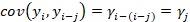
El fondo tipo 2 inicia en diciembre del 2005. Sus inversiones están distribuidas 55% en renta fija y 45% en renta variable, con un perfil balanceado destinado a trabajadores de 45 a 60 años. En la Figura 1 se observa una leve tendencia al alza con fuerte caída durante la crisis mundial entre el 2007 y el 2008; un leve descenso en abril del 2011 y 2016 en las primeras vueltas electorales, al igual que entre el 2018 y 2019, que culminó con el cierre del congreso de la República; y un fuerte retroceso en marzo del 2020 como consecuencia del COVID-19. Este desenvolvimiento corresponde al promedio mensual en soles de los valores cuota diarios para el cálculo de la rentabilidad de las AFP del fondo tipo 2.

Figura 1. Promedio mensual de los valores cuota por AFP y fondo tipo 2.
Fuente: Elaboración propia con el software Stata 16.
El presente trabajo es de gran utilidad para aquellos trabajadores de 45 a 60 años, dado que sus inversiones, al ser gestionadas por las AFP, se ven afectadas por las crisis económicas y financieras en el mundo. Como estas crisis afectan las rentabilidades del sistema privado de pensiones en el Perú, el ahorro de los trabajadores se ve afectado al momento de su jubilación. ¿Por qué las respuestas a los riesgos financieros recurrentes que adoptaron los gestores de riesgos de las AFP no mitigaron las pérdidas de la rentabilidad de la inversión de los trabajadores? Esa es la gran interrogante de los trabajadores. Con la metodología Box y Jenkins o ARIMA, se describe el comportamiento del promedio mensual de los valores diarios del fondo tipo 2 de cada AFP, así como el pronóstico de los mismos.
El objetivo de la investigación es determinar cómo se modelará adecuadamente el promedio mensual de los valores cuota por cada AFP del fondo tipo 2 con la metodología Box y Jenkins.
Asimismo, esta investigación busca determinar específicamente si la tendencia del promedio mensual de los valores cuota por cada AFP del fondo tipo 2 influye en la raíz unitaria, si la estacionariedad influye en su media y varianza, y si existe correlación entre los valores observados y los valores pronosticados.
Hipótesis específicas
1. La tendencia del promedio mensual de los valores cuota por cada AFP del fondo tipo 2 influye directamente en la raíz unitaria.
2. La estacionariedad influye directamente en la media de la rentabilidad del promedio mensual de los valores cuota por cada AFP del fondo tipo 2.
3. La estacionariedad influye directamente en la varianza de la rentabilidad del promedio mensual de los valores cuota por cada AFP del fondo tipo 2.
4. Existe correlación entre los valores observados en el promedio mensual de los valores cuota por cada AFP del fondo tipo 2 y los valores pronosticados.
Con la metodología Box y Jenkins o modelos ARIMA, se describen y pronostican los rendimientos de los promedios mensuales del valor cuota en soles del fondo tipo 2 que 4 AFP vigentes en el mercado invirtieron desde agosto del 2005 hasta julio del 2020. Los datos fueron extraídos del sitio web de la Superintendencia de Banca, Seguros y AFP, sección Boletín Estadístico de AFP (Mensual), a través del enlace https://www.sbs.gob.pe/app/stats_net/stats/EstadisticaBoletinEstadistico.aspx?p=31#. Los datos corresponden a las series de tiempo. La población para las AFP Integra y Profuturo es de 180 meses desde agosto del 2005 hasta julio del 2020; para Prima, 179 meses desde septiembre 2005 hasta julio 2020; y para Habitat, 86 meses desde junio del 2013 hasta julio del 2020. Estos datos fueron modelados con el paquete econométrico EVIEWS 10; también se recurrió al Stata 16 y Risk simulator, un software de simulación Monte Carlo que funciona como complemento de Excel. Se descartaron las AFP Horizonte y Unión Vida, dado que no se encuentran vigentes en el mercado, y se identificó la estacionariedad como un proceso estocástico estacionario en sentido débil, pues los dos primeros momentos, vale decir, la esperanza matemática y la varianza de las variables aleatorias, son constantes y no dependen del tiempo. Además, las covarianzas entre dos variables aleatorias de periodos distintos dependen solo del tiempo transcurrido entre ellas mismas, condición necesaria para que puedan ser modelados con la metodología Box y Jenkins por medio de los siguientes cuatro pasos:
En esta parte se verificó, a partir de las pruebas de raíz unitaria (RU), si las series de las cuatro AFP eran estacionarias; además, se verificó que las series tuvieran memoria o que no tuvieran ruido blanco, ya que, de lo contrario, no podrían ser pronosticadas con la metodología Box y Jenkins. Para esto, se realizaron los siguientes subpasos: análisis gráfico, cálculo de los estadísticos, pruebas de raíz unitaria y pruebas de ruido blanco.
En base a los resultados de los correlogramas, se identificaron el orden del AR y MA con el uso de la máxima verisimilitud, ensayo y error a partir de la significancia estadística de cada coeficiente estimado.
Se usó el círculo unitario para validar la estabilidad del modelo, para corroborar que los residuos y los residuos al cuadrado sean ruido blanco y, finalmente, para realizar la prueba de varianza constante con los siguientes subpasos: validación del círculo unitario, validación de los residuos y validación de los residuos al cuadrado.
Se realizó un pronóstico estático t+1, es decir, un periodo adelante, para calcular los estadísticos de error. Posteriormente se hizo un pronóstico dinámico t+k periodos.
RESULTADOS
Se presentan a continuación los resultados luego de aplicar las pruebas de la metodología Box-Jenkins, conocidas también como ARIMA.
Identificación
Análisis gráficos
Son pruebas no formales. Court y Rengifo (2011) sostienen que se determina el modelo y el orden que mejor se ajusten a los datos, puesto que se utilizan los métodos gráficos y los criterios de información. En la Figura 2 se aprecia el desenvolvimiento de las series mensuales de las AFP Habitat, Integra, Prima y Profuturo, que presentan tendencias al alza.
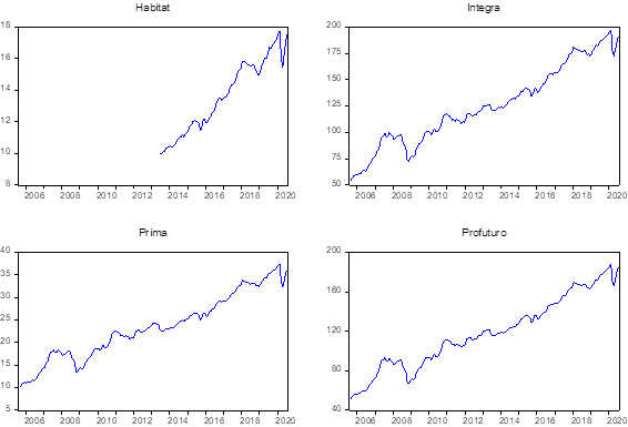
Figura 2. Comportamiento de las series promedio mensuales de las AFP Habitat, Integra, Prima y Profuturo en niveles.
Fuente: Elaboración propia con el Eviews 10.
Cálculo de los estadísticos
En la Figura 2 se aprecia que la serie original de la AFP Profuturo presenta tendencia, pero, en los resultados del modelo en la Figura 3 (lado izquierdo), tiene p-valor igual a 4.95%, es decir, menor a 5%, por lo que se rechaza la H0 de tener RU y, por lo tanto, es estacionaria; sin embargo, en la misma Figura 3 (lado derecho), se observa que la autocorrelación no decae exponencialmente para corroborar que la serie original sea estacionaria, por el contrario, esta decae linealmente, lo que indica que no es estacionaria y debe diferenciarse.
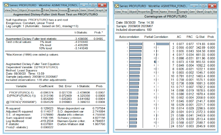
Figura 3. Cálculo de los estadísticos para la AFP Profuturo.Fuente: Elaboración propia con el Eviews 10.
Por otra parte, en la Figura 4 se aprecia que las series originales de las AFP Habitat, Integra y Prima tienen al menos una raíz unitaria y, por lo tanto, no son estacionarias. Gujarati y Porter (2010) señalan que “Por tanto, cada conjunto de datos perteneciente a la serie de tiempo corresponderá a un episodio particular. En consecuencia, no es posible generalizar para otros periodos”. Para pronosticar series temporales, las series de tiempo no estacionarias no son de mucha utilidad, y para remontar este obstáculo deberá diferenciarse las series originales para volverlas estacionarias.
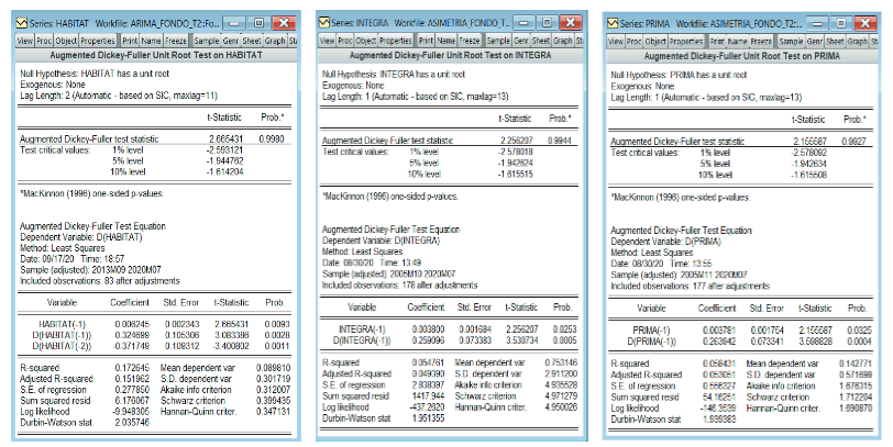
Figura 4. Cálculo de los estadísticos para las AFP Integra, Prima y Profuturo.
Fuente: Elaboración propia con Eviews 10.
Pruebas de raíz unitaria
Se realizaron las pruebas de raíz unitaria Dickey Fuller Aumentado (DFA), que según Bello (2018) son las pruebas de mayor utilización, a las series originales de Habitat, Integra, Prima y Profuturo.
Al hacer las pruebas de hipótesis a dichas series, no se rechazaron las hipótesis nulas que sugerían que las series tuvieran al menos una raíz unitaria, por lo cual, se aplicó la diferencia logarítmica de sus series originales para convertirlas en estacionarias. En la Figura 5 se muestran los resultados de los modelos.
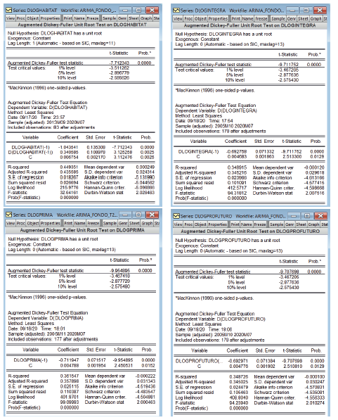
Figura 5. Pruebas de raíz unitaria.Fuente: Elaboración propia con Eviews 10.
Pruebas de ruido blanco
En esta parte se verificó que la serie de tiempo ya diferenciada tuviera memoria utilizando correlogramas y el estadístico Ljung Box (LB) para muestras pequeñas. En la Figura 6 se tienen los correlogramas para Habitat, que mostraron que hasta el mes siete no tiene ruido blanco y, a partir del mes ocho, el impacto a la serie actual de Hábitat no es significativo. En el caso de Integra, hasta el mes quince no tiene ruido blanco. Con respecto a Prima, hasta el mes trece no tiene ruido blanco. Finalmente, Profuturo no tiene ruido blanco hasta el mes dieciséis y, posterior a este mes, el impacto no es significativo en el resultado de la serie actual. En conclusión, las series diferenciadas de las AFP Habitat, Integra, Prima y Profuturo son estacionarias y no tienen ruido blanco y, por tanto, pueden pronosticarse con la metodología Box y Jenkins.
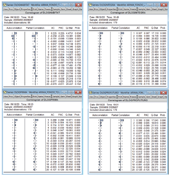
Figura 6. Pruebas de ruido blanco.
Fuente: Elaboración propia con el Eviews 10.
Estimación
Con base en los resultados de los correlogramas, se identificaron el orden del AR y MA, con el uso de la máxima verisimilitud, ensayo y error, a partir de la significancia estadística de cada coeficiente estimado. Con ayuda del software Eviews, se seleccionó automáticamente el mejor modelo, ejecutando iteraciones con combinaciones de los AR, MA y orden de integración. En este caso, se realizaron 484 modelos para cada AFP, y se eligió el modelo que tuvo el menor Akaike Info Criterion (AIC), tal como se aprecia en la Figura 7.
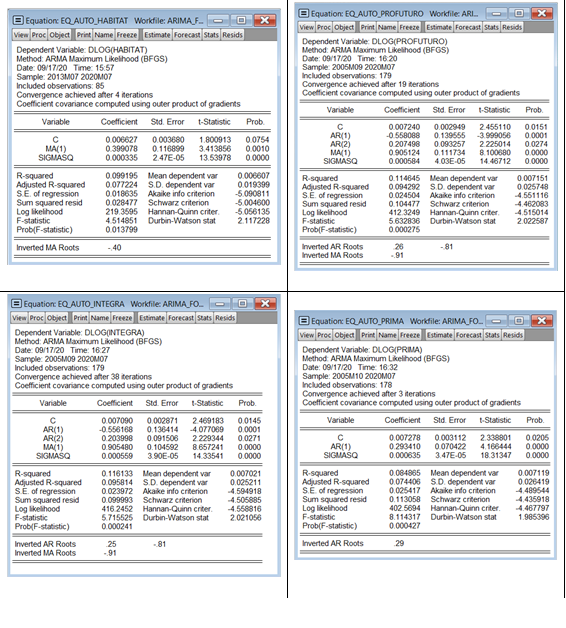
Figura 7. Identificación del orden del AR y MA.
Fuente: Elaboración propia con el Eviews 10.
Las representaciones de este modelo se aprecian en la Tabla 1 adjunta.
Tabla 1. Selección de modelos ARIMA.
|
AFP |
Representación |
|
Habitat |
ARIMA(0,1,1) |
|
Profuturo |
ARIMA(2,1,1) |
|
Integra |
ARIMA(2,1,1) |
|
Prima |
ARIMA(1,1,0) |
Fuente: Elaboración propia.
Validación
Validación de círculo unitario
Se realizó la validación con el círculo unitario y, tal como se observa en la Figura 8, los modelos son estacionarios en la parte autorregresiva para las AFP Prima, Profuturo e Integra. Asimismo, se observa que los modelos de las AFP Habitat, Profuturo e Integra son invertibles en la parte del promedio móvil. Ninguna de las raíces de las cuatro AFP está fuera del círculo unitario, y todos sus módulos están por debajo de 1, por lo que se concluye que pasaron las pruebas de validación de círculo unitario.
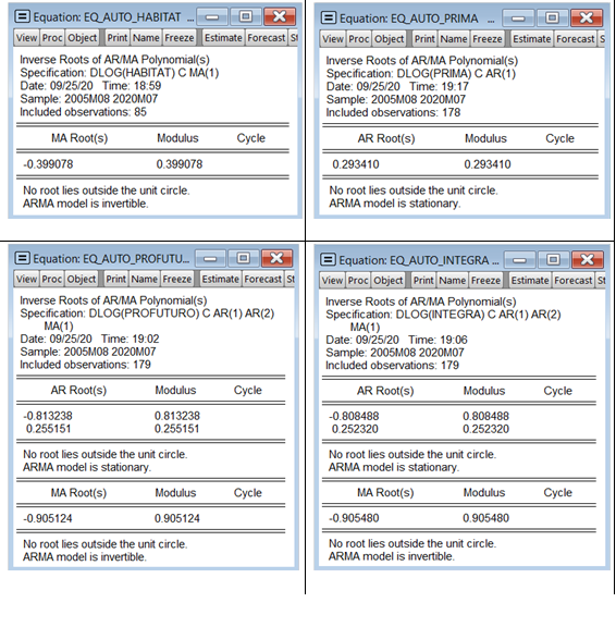
Figura 8. Validación del círculo unitario.
Fuente: Elaboración propia con el Eviews 10.
Validación de los residuos
Posteriormente, se realizó el correlograma para comprobar que los residuos tuvieran ruido blanco. En la Figura 9, se verificó que el comportamiento de los residuos de las cuatro AFP tiene ruido blanco porque sus p‑valores son mayores al 5% y, por tanto, pueden pronosticarse con los modelos ARIMA de Box y Jenkins.
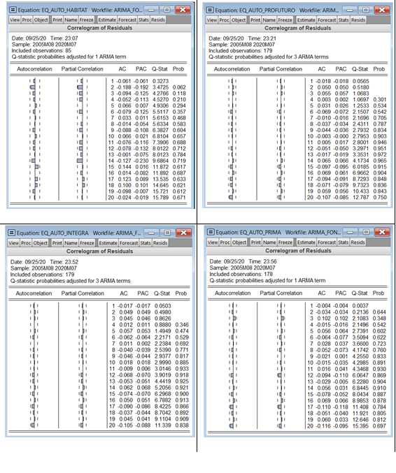
Figura 9. Validación de los residuos.
Fuente: Elaboración propia con el Eviews 10.
Validación de los residuos al cuadrado
Los residuos al cuadrado de las 4 AFP también presentaron ruido blanco, ya que todos sus p-valores están por encima del 5%, tal como se aprecia en la Figura 10; de no haber sido el caso, habría sido necesario realizar una ecuación a la varianza para luego ser trabajados con los modelos de volatilidad condicional ARCH y GARCH.
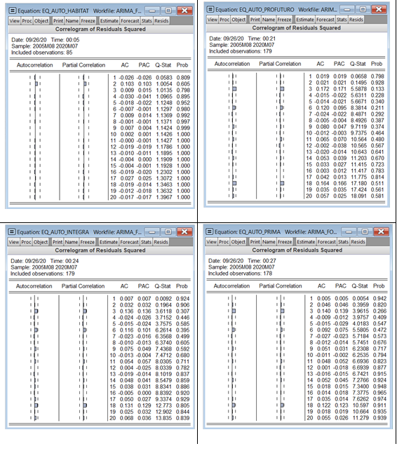
Figura 10. Validación de los residuos al cuadrado.Fuente: Elaboración propia con el Eviews 10.
Pronóstico
Curt y Rengifo (2011) sostienen que “Para determinar si un pronóstico es adecuado, se usan los estadísticos que (…) comparan los valores reales con aquellos que han sido pronosticados. (…) como los errores pueden ser positivos o negativos, (…) suma de ellos no sería de gran ayuda puesto que se cancelarían entre ellos. Es por eso que los índices trabajan ya sea con los errores al cuadrado o con el valor absoluto de los errores” (pp. 427-428); siguiendo esta línea, se pasan a realizar pronósticos estáticos del promedio mensual de los valores cuota de cada una de las cuatro AFP, a fin de tomar en cuenta los siguientes estadísticos de error: RMSE (Raíz de error cuadrático medio), MAE (Error absoluto medio), MAPE (Error Porcentual Absoluto Medio) y U-THEIL (Coeficiente de desigualdad de Theil), los cuales están contenidos en la Tabla 2.
Tabla 2. Errores de pronóstico con ARIMA.
|
|
AFP |
RMSE |
MAE |
MAPE |
U-THEIL |
|
Dentro de muestra |
Habitat |
0.2796 |
0.1665 |
1.20% |
0.8912 |
|
Profuturo |
2.6354 |
1.7516 |
1.61% |
0.9027 |
|
|
Integra |
2.8076 |
1.8535 |
1.60% |
0.9013 |
|
|
Prima |
0.5542 |
0.3582 |
1.66% |
0.9222 |
Fuente: Elaboración propia.
Se puede apreciar en la Tabla 2 que la AFP Habitat tiene el menor error de pronóstico con ARIMA, pues su RMSE, en promedio, se desvía en 0.2796 unidades y en términos porcentuales o MAPE, el desvío es 1.20%. Por su parte, la AFP Integra es la que tiene el mayor RMSE con respecto a las otras tres AFP, ya que este indica un desvío de 2.8076 unidades. En términos porcentuales, la AFP Prima tiene el mayor desvío con 1.66%.
Los pronósticos con ARIMA fueron comparados con las técnicas de suavizamiento exponencial doble contenidas en la Tabla 3, las mismas que fueron seleccionadas automáticamente de ocho técnicas por el software Risk Simulator por tener los menores estadísticos de error; estas técnicas están contenidas en la Tabla 3 y se observa que ARIMA tiene menores errores de pronóstico que el suavizamiento exponencial doble.
Tabla 3. Errores de pronóstico con técnicas de suavizamiento exponencial doble.
|
|
AFP |
RMSE |
MAE |
MAPE |
U-THEIL |
|
Dentro de muestra |
Habitat |
0.3046 |
0.0928 |
1.33% |
0.9684 |
|
Profuturo |
2.7707 |
7.6767 |
1.72% |
0.9767 |
|
|
Integra |
2.9413 |
8.6515 |
1.72% |
0.9767 |
|
|
Prima |
0.5772 |
0.3332 |
1.78% |
0.9782 |
Fuente: Elaboración propia.
Pruebas de Hipótesis
Hipótesis específica 1: La tendencia del promedio mensual de los valores cuota por cada AFP del fondo tipo 2 influye directamente en la raíz unitaria.
En la Tabla 4, se aprecia que la serie original de la AFP Profuturo no presenta tendencia y su p-valor es igual a 4.95%, menor a 5%, por lo que se rechaza la H0 de tener raíz unitaria y, por tanto, la serie es estacionaria. En la misma Tabla 4, se aprecia que los p‑valores de Habitat, Integra y Prima están por encima del 5%, entonces no se rechazan las H0, pues estas tienen al menos una raíz unitaria y no son estacionarias.
Tabla 4. Pruebas de hipótesis de raíz unitaria para las AFP Habitat, Profuturo, Integra y Prima.
Prueba de hipótesis para la AFP Habitat |
Prueba de hipótesis para la AFP Profuturo |
|
a) Hipótesis nula y alterna H0: 𝜙 = 1; x𝑡 tiene RU H1: 𝜙 < 1; x𝑡 no tiene RU |
a) Hipótesis nula y alterna Ho: 𝜙 = 1; x𝑡 tiene RU H1: 𝜙 < 1; x𝑡 no tiene RU |
b) Nivel de significancia = 0.05 |
b) Nivel de significancia = 0.05 |
c) p‑valor = 0.9980 |
c) p‑valor = 0.0495 |
Decisión: Como p‑valor = 0.9980 > 0.05 no se rechaza la H0. La serie tiene al menos una raíz unitaria. |
Decisión: Como p‑valor = 0.0495 < 0.05 se rechaza la H0. La serie original no tiene RU. |
Prueba de hipótesis para la AFP Integra |
Prueba de hipótesis para la AFP Prima |
|
a) Hipótesis nula y alterna H0: 𝜙 = 1; x𝑡 tiene RU H1: 𝜙 < 1; x𝑡 no tiene RU |
a) Hipótesis nula y alterna H0: 𝜙 = 1; x𝑡 tiene RU H1: 𝜙 < 1; x𝑡 no tiene RU |
b) Nivel de significancia = 0.05 |
b) Nivel de significancia = 0.05 |
c) p‑valor = 0.9944 |
c) p‑valor = 0.9927 |
Decisión: Como p‑valor = 0.9944 > 0.05 no se rechaza la H0. La serie tiene al menos una raíz unitaria. |
Decisión: Como p‑valor = 0.9927 > 0.05 no se rechaza la H0. La serie tiene al menos una raíz unitaria. |
Fuente: Elaboración propia.
Hipótesis específica 2: La estacionariedad influye directamente en la media de la rentabilidad del promedio mensual de los valores cuota por cada AFP del fondo tipo 2.
A cada AFP se le realizó una diferenciación, y los resultados de las pruebas de hipótesis contenidas en la Tabla 5 indican que sus p‑valores son menores al 5% y, por tanto, se rechazan las hipótesis nulas. La serie diferenciada para cada AFP no tiene raíz unitaria y por tanto es estacionaria con media constante.
Tabla 5. Prueba de hipótesis para la media de las AFP Habitat, Integra, Prima y Profuturo.
|
Prueba de hipótesis para la AFP Habitat |
Prueba de hipótesis para la AFP Integra |
|
a) Hipótesis nula y alterna H0: 𝜙 = 1; x𝑡 tiene RU H1: 𝜙 < 1; x𝑡 no tiene RU |
a) Hipótesis nula y alterna H0: 𝜙 =1; x𝑡 tiene RU H1: 𝜙 <1; x𝑡 no tiene RU |
|
b) Nivel de significancia = 0.05 |
b) Nivel de significancia = 0.05 |
|
c) p‑valor = 0.000 |
c) p‑valor = 0.000 |
|
Decisión: Como p‑valor = 0.000 < 0.05 se rechaza la H0. La serie diferenciada no tiene RU y por tanto es estacionaria. |
Decisión: Como p‑valor = 0.000 < 0.05 se rechaza la H0. La serie diferenciada no tiene RU y por tanto es estacionaria. |
|
Prueba de hipótesis para la AFP Prima |
Prueba de hipótesis para la AFP Profuturo |
|
a) Hipótesis nula y alterna H0: 𝜙 = 1; x𝑡 tiene RU H1: 𝜙 < 1; x𝑡 no tiene RU |
a) Hipótesis nula y alterna H0: 𝜙 =1; x𝑡 tiene RU H1: 𝜙 <1; x𝑡 no tiene RU |
|
b) Nivel de significancia = 0.05 |
b) Nivel de significancia = 0.05 |
|
c) p‑valor = 0.000 |
c) p‑valor = 0.000 |
|
Decisión: Como p‑valor = 0.000 < 0.05 se rechaza la H0. La serie diferenciada no tiene RU y por tanto es estacionaria. |
Decisión: Como p‑valor = 0.000 < 0.05 se rechaza la H0. La serie diferenciada no tiene RU y por tanto es estacionaria. |
Fuente: Elaboración propia.
Hipótesis específica 3: La estacionariedad influye directamente en la varianza de la rentabilidad del promedio mensual de los valores cuota por cada AFP del fondo tipo 2.
Se verifica que las series diferenciadas no tienen memoria utilizando el estadístico Ljung Box (LB) para muestras pequeñas. Las pruebas conjuntas para los residuos al cuadrado de las cuatro AFP presentan ruido blanco, pues todos sus p-valores están por encima del 5%, tal como se aprecia en la Tabla 6.
Tabla 6. Prueba de hipótesis para la varianza de las AFP Habitat, Integra, Prima y Profuturo.
|
Prueba de hipótesis para la AFP Habitat |
Prueba de hipótesis para la AFP Integra |
|
a) Hipótesis nula y alterna H0: 𝜙1 = 𝜙2 = … = 𝜙n; x𝑡 no tiene ruido blanco H1: al menos una es diferente |
a) Hipótesis nula y alterna H0: 𝜙1= 𝜙2= …=𝜙n; x𝑡 no tiene ruido blanco H1: al menos una es diferente |
|
b) Nivel de significancia = 0.05 |
b) Nivel de significancia = 0.05 |
|
c) p‑valores > 0.05 |
c) p‑valores > 0.05 |
|
Decisión: Como p-valores > 0.05 no se rechaza la H0. La serie diferenciada tiene ruido blanco y, por tanto, varianza homocedástica |
Decisión: Como p-valores > 0.05 no se rechaza la H0. La serie diferenciada tiene ruido blanco y, por tanto, varianza homocedástica |
|
Prueba de hipótesis para la AFP Prima |
Prueba de hipótesis para la AFP Profuturo |
|
a) Hipótesis nula y alterna H0: 𝜙1= 𝜙2 = … =𝜙n; x𝑡 no tiene ruido blanco H1: al menos una es diferente |
a) Hipótesis nula y alterna H0: 𝜙1= 𝜙2= … =𝜙n; x𝑡 no tiene ruido blanco H1: al menos una es diferente |
|
b) Nivel de significancia = 0.05 |
b) Nivel de significancia = 0.05 |
|
c) p‑valores > 0.05 |
c) p‑valores > 0.05 |
|
Decisión: Como p‑valores > 0.05 no se rechaza la H0. La serie diferenciada tiene ruido blanco y, por tanto, varianza homocedástica |
Decisión: Como p‑valores > 0.05 no se rechaza la H0. La serie diferenciada tiene ruido blanco y, por tanto, varianza homocedástica |
Fuente: Elaboración propia.
Hipótesis especifica 4: Existe correlación entre los valores observados del promedio mensual de los valores cuota por cada AFP del fondo tipo 2 y los valores pronosticados.
En la Tabla 7, se aprecia que los resultados de los coeficientes de correlación de los valores observados del promedio mensual de los valores cuota por cada AFP del fondo tipo 2 y los valores pronosticados corresponden a correlaciones positivas fuertes; en la tabla también están contenidos sus p‑valores.
Tabla 7. Resultados de coeficiente de correlación de Pearson.
|
|
||||||||||||||||||||||||||||||||||||||||||||||||||||||||||||
|
|
||||||||||||||||||||||||||||||||||||||||||||||||||||||||||||
Fuente: Elaboración propia.
Nota: los resultados se presentan tal como los reporta el software.
En las pruebas de hipótesis contenidas en la Tabla 8, se observa que los p‑valores de cada una de las AFP están por debajo del 5%, por tanto, además de existir una correlación fuerte y directa entre los valores observados y pronosticados, estos pueden ser corroborados con los resultados de los estadísticos de error contenidos en la Tabla 3.
Tabla 8. Pruebas de hipótesis de correlación de Pearson para las AFP Habitat, Integra, Prima y Profuturo.
|
Prueba de hipótesis para la AFP Habitat |
Prueba de hipótesis para la AFP Integra |
|
a) Hipótesis nula y alterna H0: ρ = 0 No existe correlación entre los valores observados y pronosticados H1: ρ ≠ 0 Sí existe correlación entre los valores observados y pronosticados. |
a) Hipótesis nula y alterna H0: ρ = 0 No existe correlación entre los valores observados y pronosticados H1: ρ ≠ 0 Sí existe correlación entre los valores observados y pronosticados. |
|
b) Nivel de significancia α = 0.05 |
b) Nivel de significancia α = 0.05 |
|
c) p‑valor = 0.0000 |
c) p‑valor = 0.0000 |
|
Decisión: Como p‑valor 0.0000 < 0.05, se rechaza la H0. Existe una correlación directa entre los valores observados y pronosticados. |
Decisión: Como p‑valor 0.0000 < 0.05, se rechaza la H0. Existe una correlación directa entre los valores observados y pronosticados. |
|
Prueba de hipótesis para la AFP Prima |
Prueba de hipótesis para la AFP Profuturo |
|
a) Hipótesis nula y alterna H0: ρ = 0 No existe correlación entre los valores observados y pronosticados H1: ρ ≠ 0 Sí existe correlación entre los valores observados y pronosticados |
a) Hipótesis nula y alterna H0: ρ = 0 No existe correlación entre los valores observados y pronosticados H1: ρ ≠ 0 Sí existe correlación entre los valores observados y pronosticados |
|
b) Nivel de significancia α = 0.05 |
b) Nivel de significancia α = 0.05 |
|
c) p‑valor = 0.0000 |
c) p‑valor = 0.0000 |
|
Decisión: Como p‑valor 0.0000 < 0.05 se rechaza la H0. Existe una correlación directa entre los valores observados y pronosticados. |
Decisión: Como p‑valor 0.0000 < 0.05 se rechaza la H0. Existe una correlación directa entre los valores observados y pronosticados. |
Fuente: Elaboración propia.
DISCUSIÓN
Se observó que las series originales del promedio mensual de los valores cuota por cada AFP de fondo tipo 2 presentaban tendencia y, por tanto, no eran estacionarias, por lo que se les hicieron diferencias logarítmicas para convertirlas. Esto concuerda con los resultados de las siguientes investigaciones:
- Villalba y Flores (2016) estudiaron el índice de precios y cotizaciones (IPC) del mercado bursátil mexicano y verificaron el comportamiento de la volatilidad y la importancia de que las series de este índice fueran estacionarias con el fin pronosticar los precios de las acciones que lo componen.
- Parody et al. (2016) calcularon los precios de cierre diario de las acciones del Banco de Colombia, el Banco de Bogotá y el Banco de Occidente en el periodo de tiempo comprendido entre el 17 y el 24 de julio de 2015, y obtuvieron “los rendimientos diarios de las series de cada banco estudiado mediante la diferencia obtenida entre los logaritmos neperianos de los precios actuales y los precios del día inmediatamente anterior”.
También se observó que la serie estacionaria del promedio mensual de los valores de cuota por AFP del fondo tipo 2 presenta varianza constante u homogénea, lo que significa que no presenta mucha volatilidad, de acuerdo a los siguientes hallazgos:
- Amaris et al. (2017) concluyen que “El análisis estadístico permitió tomar una decisión del modelo escogido, el cual cumple con los parámetros requeridos de normalidad, varianza constante y aleatoriedad”.
- Gallego-Nicasio et al. (2018), en uno de sus resultados, encontraron que, al efectuar la primera diferencia, la nueva serie es estacionaria, homogénea e integrada de orden uno. Sostienen que el modelo ARIMA (p,d,q) se llama proceso autorregresivo integrado de medias móviles de orden p, d, q; y que la perturbación o error se conoce como ruido blanco, siendo la media nula, la varianza homocedástica y la covarianza nula entre los choques o errores de las observaciones.
CONCLUSIONES
1. La serie original del promedio mensual de los valores cuota por AFP del fondo tipo 2 que inició en diciembre del 2005 presenta tendencia alcista durante el periodo 2005-2020.
2. Para pronosticar el promedio mensual de los valores cuota por AFP del fondo tipo 2 con los modelos Box y Jenkins o ARIMA deben eliminarse las tendencias mediante la diferenciación hasta convertir las series en estacionarias. En este caso, solo bastó con la primera diferencia.
3. Los resultados muestran que es un proceso estocástico en sentido débil porque tanto el primer como el segundo momento de la serie son invariantes a lo largo del tiempo.
4. Los retornos fueron calculados con la diferencia logarítmica del promedio del mes actual entre el promedio del mes anterior, para convertirlas en estacionarias.
5. Los modelos del retorno están en función de una media que es su comportamiento a largo plazo más un error o perturbación que desvía dicho comportamiento, pero esos errores se distribuyen como una normal y, por lo tanto, la varianza es homocedástica.
6. Con los correlogramas, el estadístico Ljung Box y el p‑valor, se validó que la serie original del promedio mensual de los valores cuota por AFP del fondo tipo 2 tuviera memoria y se concluyó que es homocedástica o de varianza constante a lo largo del tiempo, por lo que puede pronosticarse con la metodología Box y Jenkins.
7. Los residuos y los residuos al cuadrado tienen ruido blanco, y su varianza es homocedástica, por lo que pueden utilizarse la metodología Box y Jenkins.
8. Al tener varianza constante y no ser altamente volátiles, los rendimientos son conservadores y, por tanto, no satisfacen las expectativas de los trabajadores.
9. Las crisis económicas y financieras impactan negativamente en los rendimientos de la inversión de los trabajadores.
10. Los pronósticos dentro de la muestra con la metodología Box y Jenkins tienen menores errores de pronóstico que con el suavizamiento exponencial doble.
REFERENCIAS BIBLIOGRÁFICAS
[1] Amaris, G., Ávila, H., y Guerrero, T. (2017). Aplicación de modelo ARIMA para el análisis de series de volúmenes anuales en el río Magdalena. Tecnura 21(52), 88-101.
[2] Asociación de AFP. (2018). Las pensiones del SPP a los 25 años de creación. [Serie Documentos de Trabajo N°1-2018]. Lima, Perú: Asociación de AFP.
[3] Bello, M. (2018). Modelos econométricos con EViews: Modelos de regresión lineal y series de tiempo. [Apuntes de clase en línea, sesión 4]. Bogotá, Colombia: Software Shop.
[4] Box, G., Jenkins, G., y Reinsel, G. (2008). Time Series Analysis (4a ed.). Nueva Jersey, Estados Unidos: John Wiley & Sons, Inc.
[5] Court, E., y Rengifo, E. (2011). Estadísticas y Econometría Financiera. Buenos Aires, Argentina: Cengage Learning Argentina.
[6] Cruz-Saco, M., Mendoza, J., y Seminario, B. (2014). El sistema previsional del Perú: diagnóstico 1996-2013, proyecciones 2014-2050 y reforma. [Documento de discusión]. Lima, Perú: Universidad del Pacífico.
[7] Flórez, W. (2014). La administración de fondos privados de pensiones de Perú frente a las crisis financieras internacionales (1993-2013). Pensamiento Crítico, 19(2), 119-136. Recuperado de https://doi.org/10.15381/pc.v19i2.11107
[8] Gallego-Nicasio, J., Rodríguez, A., Mínguez, J., y Jiménez, F. (2018). Modelos ARIMA para la predicción del gasto conjunto de oxígeno de vuelo y otros gases en el Ejército del Aire. Sanidad Militar, 74(4), 223 - 229.
[9] Gujarati, D., y Porter, D. (2010). Econometría (5ª ed.). México D.F., México: McGraw-Hill.
[10] Gutiérrez, R., Ortiz, E. y García, O. (2017). Los efectos de largo plazo de la asimetría y persistencia en la predicción de la volatilidad: evidencia para mercados accionarios de América Latina. Contaduría y Administración, 62(4), 1063-1080. Recuperado de https://www.sciencedirect.com/science/article/pii/S0186104216300122#bbib0205
[11] Mira, P. (2016). Humano, demasiado humano. Crítica del libro "Misbehaving", de Richard Thaler. Revista de economía política de Buenos Aires, 15(10), 123-131. Recuperado de http://ojs.econ.uba.ar/index.php/REPBA/article/view/1159
[12] Ñaupas, H., Mejía, E., Novoa, E., y Villagómez, A. (2014). Metodología de la investigación (4ª ed.). Bogotá, Colombia: Ediciones de la U.
[13] Ortiz, I., Durán-Valverde, F., Urban, S., Wodsak, V., y Yu, Z. (2019). La privatización de las pensiones: tres décadas de fracasos. El trimestre económico, LXXXVI 3(343), 799-838. Recuperado de https://doi.org/10.20430/ete.v86i343.926
[14] RTV San Marcos - UNMSM. (5 de agosto de 2020). El modelo de AFP: Problemática y planteamientos alternativos [Video]. Youtube. Recuperado de https://www.youtube.com/watch?v=wKf6wqOB1rw&feature=emb_title
[15] Parody, E., Charris, A., y García, R. (2016). Modelo Log-normal para predicción del precio de las acciones del sector bancario que cotizan en el Índice General de la Bolsa de Valores de Colombia. Dimensión Empresarial, 14(1), 137-149.
[16] Ramón, N., y López, J. (2016). Econometría series temporales y modelos de ecuaciones simultáneas. Elche, España: Universidad Miguel Hernández.
[17] Villalba, F., y Flores-Ortega, M. (2016). Análisis de la volatilidad del índice principal del mercado bursátil mexicano, del índice de riesgo país y de la mezcla mexicana de exportación mediante un modelo GARCH trivariado asimétrico. Revista de Métodos Cuantitativos para la Economía y la Empresa, 17, 3-22. Recuperado de https://www.upo.es/revistas/index.php/RevMetCuant/article/view/2191
Revista Industrial Data 24(1): 243-276 (2021)
DOI: https://dx.doi.org/10.15381/idata.v24i1.18930
ISSN: 1560-9146 (Impreso) / ISSN: 1810-9993 (Electrónico)
Received: 22/10/2020 Accepted: 07/12/2020 Published: 26/07/2021
Modeling the Monthly Average of the Quota Values per AFP and Type 2 Fund with the Box and Jenkins or ARIMA Methodology
Wilfredo Bazán Ramírez[2]
ABSTRACT
The economic and financial crises in the world are recurrent due to the presentation of different patterns. These crises have affected the returns of the private pension system in Peru and there were no effective responses from the Pension Fund Administrators (AFPs). By using the Box and Jenkins or Autoregressive Integrated Moving Average (ARIMA) methodology, the behavior of the monthly average returns of the daily quota values of the type 2 fund—which began in December 2005—of each AFP can be described and forecast. Type 2 funds are distributed 55% in fixed income and 45% in equities, with a balanced profile destined for workers between 45 and 60 years old. The data type of the monthly average returns of the type 2 fund corresponds to the weak stationary time series, since the first moments such as the mean and the variance and autocovariance are time‑invariant.
Key words: time series, profitability, weak stationarity, unit root, white noise.
INTRODUCTION
The Box and Jenkins or Autoregressive Integrated Moving Average (ARIMA) methodology was used to describe and forecast the behavior of the returns of the monthly average of the quota values of the type 2 fund—which began in December 2005—of each AFP. The type of data of the monthly returns of the type 2 fund corresponds to time series and, in order to be modeled with ARIMA, they must be weak‑sense stationary, where the first two moments as the mean, and the variance and autocovariance must be time‑invariant.
In 1976, Box and Jenkins formalized the Box-Jenkins methodology and ARIMA models (also known as Box-Jenkins models) where they mentioned time series that are supported by stochastic processes (Box, Jenkins & Reinsel, 2008). When forecasting with an ARIMA model, the following steps need to be followed:
1. Identification
2. Estimation
3. Diagnostic checking
4. Forecasting
These steps are shown in Box et al. (2008), where they are referred to as “Stages in the iterative approach to model building” (p.18).
Gujarati and Porter (2010) argue that when a time series is not stationary, the mean and variance are not time‑invariant. Moreover, when referring to the Box and Jenkins methodology ARIMA, they add the following:
The publication by Box and Jenkins of Time Series Analysis: Forecasting and Control (op. cit.) ushered in a new generation of forecasting tools. Popularly known as the Box–Jenkins (BJ) methodology, but technically known as the ARIMA methodology, the emphasis of these methods is not on constructing single-equation or simultaneous-equation models but on analyzing the probabilistic, or stochastic, properties of economic time series on their own (...). Unlike the regression models, in which Yt is explained by k regressors X1, X2, X3, ..., Xk, the BJ-type time series models allow Yt to be explained by past, or lagged, values of Y itself and stochastic error terms. For this reason, ARIMA models are sometimes called atheoretic models because they are not derived from any economic theory. (pp. 774-775).
Court and Rengifo (2011) state that El concepto de estacionariedad tiene dos versiones: la estacionariedad estricta y la estacionariedad débil [The concept of stationarity has two versions: strict stationarity and weak stationarity] (p. 400); each of these is shown below:
Strict Stationarity. It is a stochastic process {yi} with i = 1, 2, …, T. It is strictly stationary if, for a finite real number R and for any set of subscripts i1, i2, …, iT, it is defined as follows:
Weak Stationarity. It is a stochastic process {yi} with i = 1, 2, …, T. It is weakly stationary if the meets the following:
Ramon and Lopez (2016) also identify two types of stationarity: strong-sense and weak-sense. For the first case, the four moments of the joint distributions are time-invariant, and for the second, only the first 2 moments are. In this case, the Box and Jenkins methodology is based on weak-sense stationarity.
Problematic Situation
Ñaupas et al. (2014) indicate that in daily life there are repetitive patterns, with certain different characteristics, and that the prediction of natural phenomena is more accurate than social phenomena:
Así por ejemplo, conociendo las leyes de Kepler, que explican los movimientos de traslación de los planetas, satélites, cometas y asteroides es posible calcular la ocurrencia de eclipses, mareas y acercamiento de cometas a la órbita de la Tierra. La predicción del tiempo, de inundaciones, terremotos, huracanas, erupciones volcánicas, la ocurrencia de mareas, o de pandemias son más confiables que las ocurrencias de revoluciones, conflictos sociales, golpes de estado, etc. [Thus, for example, knowing Kepler's laws, which explain the translational movements of planets, satellites, comets and asteroids, it is possible to calculate the occurrence of eclipses, tides and approach of comets to the Earth's orbit. The prediction of the weather, floods, earthquakes, hurricanes, volcanic eruptions and the occurrence of tides, or pandemics are more reliable than the occurrence of revolutions, social conflicts, coups d'état, etc.]. (section 2.4.2. ¿Qué es la investigación natural?)
These phenomena, that originate crises, impact economies and finances in a negative way, which is why Mira (2016) considers the recurrent occurrence of financial crises. These crises have repeatedly affected the returns of the private pension system in Peru.
The International Labor Organization (ILO) established in 1933 the Convention on Old-Age Insurance, and in 1952 determined the guidelines for old-age benefits. In Peru the National Pension System (SNP), which is currently administered by the Pension Standardization Office (ONP) operated in the beginning. Between 1981 and 2014, as noted by Ortiz, Durán-Valverde, Urban, Wodsak, and Yu (2019), about 30 countries fully or partially privatized their mandatory public pensions, a fact that occurred in Peru in 1993. The Asociación de Administradoras de Fondo de Pensiones[3] (2018) defines the pension in the Peruvian private pension system (SPP) as el ingreso periódico que recibe el afiliado como consecuencia de un proceso previo de suavización de consumo, a través del ahorro a lo largo de su vida laboral en su cuenta de capitalización individual (CIC) [the periodic income received by the member as a consequence of a previous process of consumption smoothing, through savings throughout his working life in his individual capitalization account (CIC)] (p. 8) with the purpose of ensuring that the retired worker does not face economic difficulties.
AFPs are responsible for managing the contributions of each individual during his working life, that is, they invest their savings in order to obtain a return so that, once retired, the individual can enjoy their contributions and earnings with no need to depend on their family or the State. However, Cruz-Saco et al. (2014) pointed out that the pension system in Peru was ineficiente, tiene una baja probabilidad de incrementar apreciablemente la cobertura en los siguientes 36 años, y presenta, además, un conjunto de inequidades en la asignación de los beneficios previsionales [inefficient, has a low probability of appreciably increasing coverage in the next 36 years, and also presents a set of inequities in the allocation of pension benefits] (p. 2).
Flórez (2014) also adds that los ahorros para la jubilación de millones de personas se encuentran expuestos, de manera intrínseca, al comportamiento favorable, así como adverso, de los mercados financieros [the retirement savings of millions of people are intrinsically exposed to the favorable and adverse behavior of financial markets] (p. 121). These situations are the cause of high volatility, especially when there is more negative news than positive, so an asymmetric behavior of the market, especially the equity market, is observed.
Ortiz et al. (2019) argue that Los trabajadores se convirtieron así en consumidores obligados del sector financiero, con lo que asumían individualmente todos los riesgos del mercado financiero sin contar con la suficiente información para tomar decisiones sensatas [Workers became forced consumers of the financial sector, thus individually assuming all the risks of the financial market without enough information to make reliable decisions] (p. 803). In other words, when the market is stable or when there is good news, returns will be positive. On the other hand, according to Yang et al. (as cited in Gutiérrez et al., 2017), financial crises have been characterized by the increase of risk and high volatility, which has negatively affected returns. In the case of the SPP, as a consequence of negative news, the high expectations the SPP initially generated were diluted as the years went by because it did not produce the expected results.
Carlos Palomino, in an interview with RTV San Marcos - UNMSM (2020), stated that the investments of AFPs go into stock-market mechanisms and not into tangible assets. These stock-market instruments are volatile due to economic shocks or cycles which, in turn, are a consequence of external variables, such as, for example, a pandemic.
It should be noted that in November 2006, the absorption of AFP Unión Vida by Prima AFP was authorized. In April 2013, AFP Horizonte was acquired by AFP Integra and Profuturo (50% each). AFP Habitat began operations in April 2013.
The type 2 fund began operations in December 2005. Its investments are distributed 55% in fixed income and 45% in equities, with a balanced profile aimed at workers aged 45 to 60. Figure 1 shows a slight upward trend with a sharp drop during the world crisis between 2007 and 2008; a slight drop in April 2011 and 2016 during the first electoral rounds, as well as between 2018 and 2019, which culminated with the dissolution of the Congress of the Republic of Peru; and a sharp decline in March 2020 as a result of COVID-19. This performance corresponds to the monthly average in soles of the daily quota values used for calculating the profitability of the AFPs of type 2 fund.
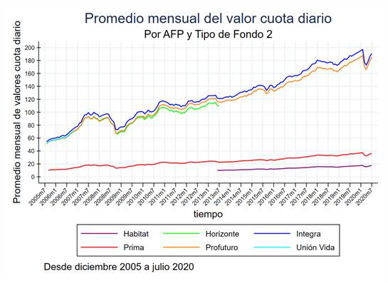
Figure 1. Monthly average of quota values for each AFP and type 2 fund.
Source: Prepared by the author using Stata 16.
This work is very useful for workers between 45 and 60 years old, since their investments, managed by the AFPs, are affected by the economic and financial crises in the world. As these crises affect the returns of the Peruvian private pension system, the savings of workers are affected at the time of their retirement. Why did the response to recurrent financial risks adopted by the risk managers of AFPs not mitigate the loss of investment returns of workers? That is the big question asked by workers. Using the Box and Jenkins or ARIMA methodology, the behavior of the monthly average of the daily values of the type 2 fund for each AFP is described, as well as their forecast.
The objective of this research is to determine how to adequately model the monthly average of the quota values for each AFP of the type 2 fund with the Box and Jenkins methodology.
Moreover, this research specifically seeks to determine if the trend of the monthly average of the quota values for each AFP of the type 2 fund influences the unit root, if stationarity influences its mean and variance, and if there is correlation between the observed values and the forecast values.
General Hypothesis
The monthly average of the quota values for each AFP of the type 2 fund will be adequately modeled with the Box and Jenkins methodology.
Specific Hypotheses
1. The trend of the monthly average of the quota values for each AFP of the type 2 fund directly influences the unit root.
2. Stationarity directly influences the mean of the return of the monthly average of the quota values for each AFP of the type 2 fund.
3. Stationarity directly influences the variance of the return of the monthly average of the quota values for each AFP of the type 2 fund.
4. There is a correlation between the observed values in the monthly average of the quota values for each AFP of the type 2 fund and the predicted values.
METHODOLOGY
Box and Jenkins methodology or ARIMA models were used to describe and forecast the returns of the monthly averages of quota values in soles of the type 2 fund that 4 AFPs—currently in the market—invested from August 2005 to July 2020. The data were extracted from the website of the Superintendencia de Banca, Seguros y AFP[4], section Boletín Estadístico de AFP[5] (Monthly), through the link https://www.sbs.gob.pe/app/stats_net/stats/EstadisticaBoletinEstadistico.aspx?p=31#. The data correspond to the time series. The population for AFP Integra and Profuturo is 180 months from August 2005 to July 2020; for Prima, 179 months from September 2005 to July 2020; and for Habitat, 86 months from June 2013 to July 2020. These data were modeled with the econometric package EVIEWS 10; Stata 16 and Risk simulator—a Monte Carlo simulation software that works as an Excel add-in—were also used. AFP Horizonte and Unión Vida were discarded, since they are not currently in the market, and stationarity was identified as a weakly stationary stochastic process, since the first two moments—the mathematical expectation and the variance of the random variables—are constant and do not depend on time. Moreover, the covariances between two random variables of different periods depend only on the time elapsed between them, a necessary condition for them to be modeled with the Box and Jenkins methodology by means of the following four steps:
Identification
In this part, it was verified, based on the unit root (UR) tests, whether the series of the four AFPs were stationary; in addition, it was verified that the series had memory or that they did not have white noise, since otherwise, they could not be forecast with the Box and Jenkins methodology. For this, the following substeps were performed: graphical analysis, statistics calculations, unit root tests and white noise tests.
Estimation
Based on the results of the correlograms, the order of the AR and MA were identified using maximum likelihood estimation and the trial and error method from the statistical significance of each estimated coefficient.
Diagnostic Checking
The unit circle was used to validate the stability of the model, to corroborate that the residuals and squared residuals are white noise, and finally to perform the constant variance test with the following substeps: validation of the unit circle, validation of the residuals, and validation of the squared residuals.
Forecasting
A static forecast t+1—that is, one period ahead—was performed to calculate the error statistics. Subsequently, a dynamic forecast t+k periods was performed.
RESULTS
The results after applying the Box-Jenkins methodology tests, also known as ARIMA, are presented below.
Identification
Graphical Analysis
These are non-formal tests. Court and Rengifo (2011) argue that they help to determine the model and the order that best fit the data, since graphical methods and information criteria are used. Figure 2 shows the development of the monthly series of AFP Habitat, Integra, Prima and Profuturo, which show upward trends.
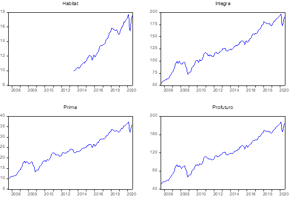
Figure 2. Behavior of the monthly average series of AFP Habitat, Integra, Prima and Profuturo by levels.
Source: Prepared by the author using Eviews 10
Statitics Calculation
Figure 2 shows that the original series of AFP Profuturo has a trend, but, in the results of the model in Figure 3 (left side), it has a p-value of 4. 95%, that is, less than 5%, so the H0 (which states that the series has a UR) is rejected and, therefore, it is stationary; however, in the same Figure 3 (right side), it can be observed that the autocorrelation does not decay exponentially to corroborate that the original series is stationary; on the contrary, it decays linearly, which indicates that it is not stationary and must be differentiated.
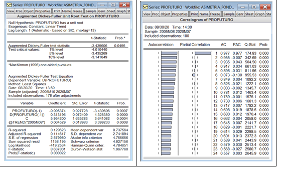
Figure 3. Statistics Calculation for AFP Profuturo.
Source: Prepared by the author using Eviews 10.
Figure 4 shows that the original series of AFP Habitat, Integra and Prima have at least one UR and, therefore, are not stationary. Gujarati and Porter (2010) point out that “Each set of time series data will therefore be for a particular episode. As a consequence, it is not possible to generalize it to other time periods”. For forecasting time series, non-stationary time series are not very useful, and to overcome this obstacle, the original series must be differentiated to make them stationary.
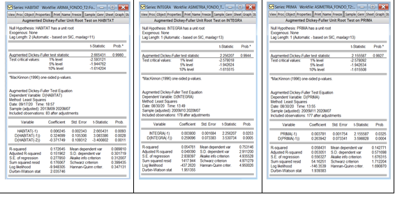
Figure 4. Statistics Calculation for AFP Integra, Prima and Profuturo.
Source: Prepared by the author using Eviews 10.
Unit Root Tests
Dickey Fuller Augmented (DFA) tests, which according to Bello (2018) are the test most widely used, were performed on the original series of Habitat, Integra, Prima and Profuturo.
When performing the hypothesis tests to those series, the null hypotheses that suggested that the series have at least one UR were not rejected, therefore, the logarithmic differentiation of their original series was applied to make them stationary. Figure 5 shows the results of the models.
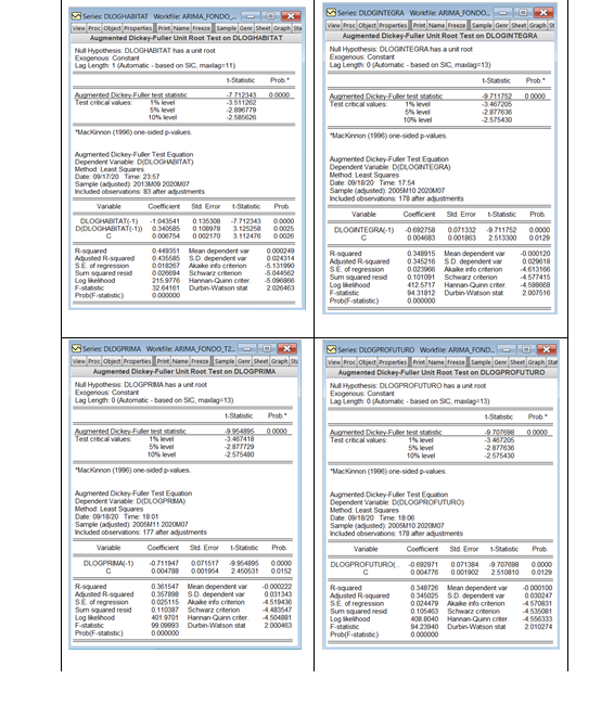
Figure 5. Unit root tests.
Source: Prepared by the author using Eviews 10.
White Noise Tests
It was verified that the time series already differentiated had memory using correlograms and the Ljung Box (LB) statistic for small samples. Figure 6 shows the correlograms for Habitat, which showed that up to month seven there is no white noise and, from month eight, the impact on the current Habitat series is not significant. In the case of Integra, there is no white noise up to month fifteen. As for Prima, there is no white noise up to month thirteen. Finally, Profuturo has no white noise until month sixteen and, after this month, the impact is not significant in the result of the current series. In conclusion, the differentiated series of AFP Habitat, Integra, Prima and Profuturo are stationary and have no white noise and, therefore, can be forecast with the Box and Jenkins methodology.
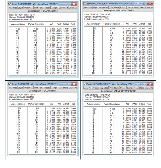
Figure 6. White noise tests.
Source: Prepared by the author using Eviews 10.
Estimation
Based on the results of the correlograms, the order of the AR and MA were identified using maximum likelihood estimation, and the trial and error method, based on the statistical significance of each estimated coefficient. Using Eviews software, the best model was automatically selected by running iterations with combinations of the AR, MA and order of integration. In this case, 484 models were run for each AFP, and the model with the lowest Akaike Info Criterion (AIC) was chosen, as shown in Figure 7.
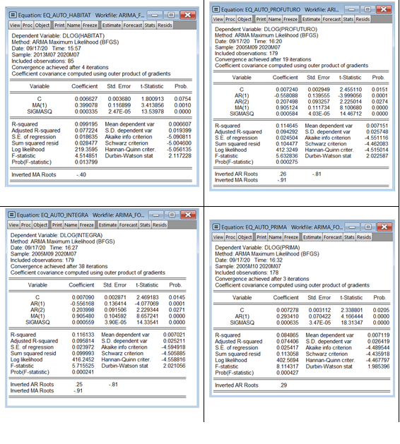
Figure 7. Identification of the order of AR and MA.
Source: Prepared by the author using Eviews 10.
The representations of this model are shown in Table 1.
Table 1. Selection of ARIMA Models.
|
AFP |
Representation |
|
Habitat |
ARIMA (0,1,1) |
|
Profuturo |
ARIMA (2,1,1) |
|
Integra |
ARIMA (2,1,1) |
|
Prima |
ARIMA (1,1,0) |
Source: Prepared by the author.
Validation
Unit Circle Validation
The validation with the unit circle was performed and, as shown in Figure 8, it can be seen that the models are stationary in the autoregressive part for AFP Prima, Profuturo and Integra. It is also observed that the models of AFP Habitat, Profuturo and Integra are invertible in the moving average part. None of the roots of the four AFPs are outside the unit circle, and all their moduli are below 1, so it is concluded that they passed the unit circle validation tests.
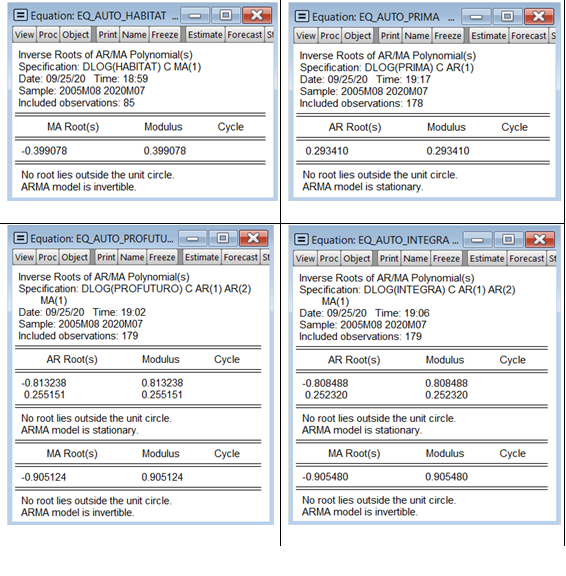
Figure 8. Unit circle validation.
Source: Prepared by the author using Eviews 10.
Validation of the residuals
Subsequently, the correlogram was performed to verify that the residuals had white noise. In Figure 9, it was verified that the behavior of the residuals of the four AFPs has white noise because their p-values are greater than 5% and, therefore, forecasting with the Box and Jenkins ARIMA models is possible.
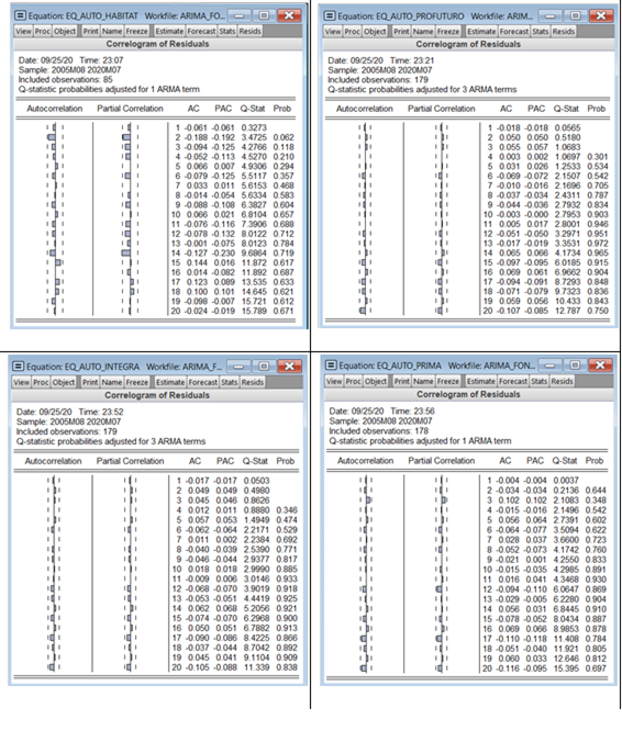
Figure 9. Validation of the residuals.
Source: Prepared by the author using Eviews 10.
Validation of the squared residuals
The squared residuals of the 4 AFPs also presented white noise, since all their p‑values are above 5%, as shown in Figure 10; if this had not been the case, it would have been necessary to perform an equation to the variable and then work with the conditional volatility models ARCH and GARCH.
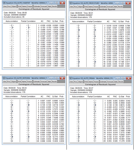
Figure 10. Validation of the squared residuals.
Source: Prepared by the author using Eviews 10.
Forecasting
Curt and Rengifo (2011) argue that Para determinar si un pronóstico es adecuado, se usan los estadísticos que (…) comparan los valores reales con aquellos que han sido pronosticados. (…) como los errores pueden ser positivos o negativos, (…) suma de ellos no sería de gran ayuda puesto que se cancelarían entre ellos. Es por eso que los índices trabajan ya sea con los errores al cuadrado o con el valor absoluto de los errores [To determine whether a forecast is adequate, statistics that (...) compare actual values with those that have been predicted are used. (...) as errors can be positive or negative, (...) to use addition with them would not be of great help since they would cancel each other. That is why the indices work either with squared errors or with the absolute value of the errors] (pp. 427-428); so static forecasts of the monthly average of the quota values of each of the four AFPs are performed in order to take into account the following error statistics: RMSE (Root Mean Square Error), MAE (Mean Absolute Error), MAPE (Mean Absolute Percentage Error) and U-THEIL (Theil’s Inequality Coefficient), which are contained in Table 2.
Table 2. Forecast Errors with ARIMA.
|
|
AFP |
RMSE |
MAE |
MAPE |
U-THEIL |
|
In sample |
Habitat |
0.2796 |
0.1665 |
1.20% |
0.8912 |
|
Profuturo |
2.6354 |
1.7516 |
1.61% |
0.9027 |
|
|
Integra |
2.8076 |
1.8535 |
1.60% |
0.9013 |
|
|
Prima |
0.5542 |
0.3582 |
1.66% |
0.9222 |
Source: Prepared by the author.
Table 2 shows that AFP Habitat has the lowest forecast error with ARIMA, since its RMSE, on average, deviates by 0.2796 units and in percentage terms or MAPE, the deviation is 1.20%. AFP Integra has the highest RMSE with respect to the other three AFPs, with a deviation of 2.8076 units. In percentage terms, AFP Prima has the highest deviation with 1.66%.
The forecasts with ARIMA were compared with the double exponential smoothing techniques contained in Table 3, which were automatically selected out of eight techniques by the Risk Simulator software for having the lowest error statistics; these techniques are contained in Table 3 and it is observed that ARIMA has lower forecast errors than double exponential smoothing.
Table 3. Forecast Errors with Double Exponential Smoothing Techniques.
|
|
AFP |
RMSE |
MAE |
MAPE |
U-THEIL |
|
In sample |
Habitat |
0.3046 |
0.0928 |
1.33% |
0.9684 |
|
Profuturo |
2.7707 |
7.6767 |
1.72% |
0.9767 |
|
|
Integra |
2.9413 |
8.6515 |
1.72% |
0.9767 |
|
|
Prima |
0.5772 |
0.3332 |
1.78% |
0.9782 |
Source: Prepared by the author.
Hypothesis Testing
Specific hypothesis 1: The trend of the monthly average of the quota values for each AFP of the type 2 fund directly influences the unit root.
Table 4 shows that the original series of AFP Profuturo does not show a trend and its p-value is equal to 4.95%, less than 5%, so the H0 (which states that the series has a UR) is rejected and, therefore, the series is stationary. Table 4 also shows that the p-values of Habitat, Integra and Prima are above 5%, so the H0s are not rejected since they have at least one UR and are not stationary.
Table 4. Unit Root Hypothesis Tests for AFPs Habitat, Profuturo, Integra and Prima.
Hypothesis test for AFP Habitat |
Hypothesis test for AFP Profuturo |
|
a) Null and alternate hypothesis H0: 𝜙 = 1; x𝑡 has UR H1: 𝜙 < 1; x𝑡 has no UR |
a) Null and alternate hypothesis Ho: 𝜙 = 1; x𝑡 has UR H1: 𝜙 < 1; x𝑡 has no UR |
b) Significance level = 0.05 |
b) Significance level = 0.05 |
c) p‑value = 0.9980 |
c) p‑value = 0.0495 |
Decision: As p‑value = 0.9980 > 0.05, H0 is not rejected. The series has at least one UR. |
Decision: As p‑value = 0.0495 < 0.05, H0 is rejected. The original has no UR. |
Hypothesis test for AFP Integra |
Hypothesis test for AFP Prima |
|
a) Null and alternate hypothesis H0: 𝜙 = 1; x𝑡 has UR H1: 𝜙 < 1; x𝑡 has no UR |
a) Null and alternate hypothesis H0: 𝜙 = 1; x𝑡 has UR H1: 𝜙 < 1; x𝑡 has no UR |
b) Significance level = 0.05 |
b) Significance level = 0.05 |
c) p-value = 0.9944 |
c) p-value = 0.9927 |
Decision: As p‑value = 0.9944 > 0.05, H0 is not rejected. The series has at least one UR. |
Decision: As p‑value = 0.9927 > 0.05, H0 is not rejected. The series has at least one UR. |
Source: Prepared by the author.
Specific hypothesis 2: Stationarity has a direct influence on the mean of the return of the monthly average of the quota values for each AFP of type 2 fund.
A differentiation was made for each AFP, and the results of the hypothesis tests contained in Table 5 indicate that their p-values are less than 5% and, therefore, the null hypotheses are rejected. The differentiated series for each AFP has no unit root and is therefore stationary with constant mean.
Table 5. Hypothesis Test for the Mean of AFPs Habitat, Integra, Prima and Profuturo.
|
Hypothesis test for AFP Habitat |
Hypothesis test for AFP Integra |
|
a) Null and alternate hypothesis H0: 𝜙 = 1; x𝑡 has UR H1: 𝜙 < 1; x𝑡 has no UR |
a) Null and alternate hypothesis H0: 𝜙 =1; x𝑡 has UR H1: 𝜙 <1; x𝑡 has no UR |
|
b) Significance level = 0.05 |
b) Significance level = 0.05 |
|
c) p-value = 0.000 |
c) p-value = 0.000 |
|
Decision: As p‑value = 0.000 < 0.05, H0 is rejected. The differentiated series has no RU and is therefore stationary. |
Decision: As p‑value = 0.000 < 0.05, H0 is rejected. The differentiated series has no RU and is therefore stationary. |
|
Hypothesis test for AFP Prima |
Hypothesis test for AFP Profuturo |
|
a) Null and alternate hypothesis H0: 𝜙 = 1; x𝑡 has UR H1: 𝜙 < 1; x𝑡 has no UR |
a) Null and alternate hypothesis H0: 𝜙 =1; x𝑡 has UR H1: 𝜙 <1; x𝑡 has no UR |
|
b) Significance level = 0.05 |
b) Significance level = 0.05 |
|
c) p-value = 0.000 |
c) p-value = 0.000 |
|
Decision: As p‑value = 0.000 < 0.05, H0 is rejected. The differentiated series has no RU and is therefore stationary. |
Decision: As p‑value = 0.000 < 0.05, H0 is rejected. The differentiated series has no RU and is therefore stationary. |
Source: Prepared by the author.
Specific hypothesis 3: Stationarity directly influences the variance of the return of the monthly average of the quota values for each AFP of the type 2 fund.
It is verified that the differentiated series have no memory using the Ljung Box (LB) statistic for small samples. The joint tests for the squared residuals of the four AFPs present white noise, since all their p-values are above 5%, as shown in Table 6.
Table 6. Hypothesis Test for the Variance of AFPs Habitat, Integra, Prima and Profuturo.
|
Hypothesis test for AFP Habitat |
Hypothesis test for AFP Integra |
|
a) Null and alternate hypothesis H0: 𝜙1 = 𝜙2 = … = 𝜙n; x𝑡 has no white noise H1: at least one is different |
a) Null and alternate hypothesis H0: 𝜙1= 𝜙2= …=𝜙n; x𝑡 has no white noise H1 at least one is different |
|
b) Significance level = 0.05 |
b) Significance level = 0.05 |
|
c) p‑values > 0.05 |
c) p‑values > 0.05 |
|
Decision: As p‑values > 0.05, H0 is not rejected. The differentiated series has white noise and, therefore, homoscedastic variance. |
Decision: As p‑values > 0.05, H0 is not rejected. The differentiated series has white noise and, therefore, homoscedastic variance. |
|
Hypothesis test for AFP Prima |
Hypothesis test for AFP Profuturo |
|
a) Null and alternate hypothesis H0: 𝜙1= 𝜙2 = … =𝜙n; x𝑡 has no white noise H1: at least one is different |
a) Null and alternate hypothesis H0: 𝜙1= 𝜙2= … =𝜙n; x𝑡 has no white noise H1: at least one is different |
|
b) Significance level = 0.05 |
b) Significance level = 0.05 |
|
c) p‑values > 0.05 |
c) p‑values > 0.05 |
|
Decision: As p‑values > 0.05, H0 is not rejected. The differentiated series has white noise and, therefore, homoscedastic variance. |
Decision: As p‑values > 0.05, H0 is not rejected. The differentiated series has white noise and, therefore, homoscedastic variance. |
Source: Prepared by the author.
Specific hypothesis 4: There is a correlation between the observed values of the monthly average of the quota values for each AFP of the type 2 fund and the predicted values.
Table 7 shows that the results of the correlation coefficients of the observed values of the monthly average of the quota values for each AFP of the type 2 fund and the predicted values correspond to strong positive correlations; the table also contains their p-values.
Table 7. Results of Pearson's correlation coefficient.
|
|
||||||||||||||||||||||||||||||||||||||||||||||||||||||||||||
|
|
||||||||||||||||||||||||||||||||||||||||||||||||||||||||||||
Soure: Prepared by the author.
Note: the results are presented as reported by the software.
In the hypothesis tests contained in Table 8, it is observed that the p-values of each AFP are below 5%, therefore, in addition to the strong and direct correlation between the observed and predicted values, these can be corroborated with the results of the error statistics contained in Table 3.
Table 8. Hypothesis tests for Pearson’s correlation of AFP Habitat, Integra, Prima and Profuturo.
|
Hypothesis test for AFP Habitat |
Hypothesis test for AFP Integra |
|
a) Null and alternate hypothesis H0: ρ = 0 There is no correlation between the observed and predicted values. H1: ρ ≠ 0 There is a correlation between the observed and predicted values. |
a) Null and alternate hypothesis H0: ρ = 0 There is no correlation between the observed and predicted values. H1: ρ ≠ 0 There is a correlation between the observed and predicted values. |
|
b) Significance level = 0.05 |
b) Significance level = 0.05 |
|
c) p‑value = 0.0000 |
c) p‑value = 0.0000 |
|
Decision: As p‑value 0.0000 < 0.05, H0 is rejected. There is a direct correlation between the observed and forecast values. |
Decision: As p‑value 0.0000 < 0.05, H0 is rejected. There is a direct correlation between the observed and forecast values. |
|
Hypothesis test for AFP Prima |
Hypothesis test for AFP Profuturo |
|
a) Null and alternate hypothesis H0: ρ = 0 There is no correlation between the observed and predicted values H1: ρ ≠ 0 There is a correlation between the observed and predicted values. |
a) Null and alternate hypothesis H0: ρ = 0 There is no correlation between the observed and predicted values H1: ρ ≠ 0 There is a correlation between the observed and predicted values. |
|
b) Significance level = 0.05 |
b) Significance level = 0.05 |
|
c) p‑value = 0.0000 |
c) p‑value = 0.0000 |
|
Decision: As p‑value 0.0000 < 0.05, H0 is rejected. There is a direct correlation between the observed and forecast values. |
Decision: As p‑value 0.0000 < 0.05, H0 is rejected. There is a direct correlation between the observed and forecast values. |
Source: Prepared by the author.
DISCUSSION
It was observed that the original series of the monthly average of the quota values for each type 2 fund AFP had a trend and, therefore, were not stationary, so logarithmic differentiations were made to convert them. This is consistent with the results of the following research:
- Villalba and Flores (2016) studied the price and quotes index (IPC) of the Mexican stock market and verified the behavior of the volatility and the importance of the stationarity of its series for forecasting the prices of the stocks that compose it.
- Parody et al. (2016) calculated the daily closing prices of the shares of Banco de Colombia, Banco de Bogotá and Banco de Occidente between July 17 and 24, 2015, and obtained los rendimientos diarios de las series de cada banco estudiado mediante la diferencia obtenida entre los logaritmos neperianos de los precios actuales y los precios del día inmediatamente anterior [the daily returns of the series of each bank studied through the difference of the neperian logarithms of the current prices and the prices of the immediately preceding day].
It was also observed that the stationary series of the monthly average of the quota values for each AFP of the type 2 fund presents constant or homogeneous variance, which means that it does not present much volatility, according to the following findings:
- Amaris et al. (2017) conclude that el análisis estadístico permitió tomar una decisión del modelo escogido, el cual cumple con los parámetros requeridos de normalidad, varianza constante y aleatoriedad [The statistical analysis made it possible to make a decision on the chosen model, which complies with the required parameters of normality, constant variance and randomness].
- Gallego-Nicasio et al. (2018) found in one of their results that, when performing the first differentiation, the new series is stationary, homogeneous and integrated of order one. They say that the ARIMA (p,d,q) model is called Autoregressive Integrated Moving Average process of order p, d, q; and that the disturbance or error is known as white noise, with the mean being zero, the variance homocedastic and the covariance null among the shocks or errors of the observations.
CONCLUSIONS
1. The original series of the monthly average of the AFP quota values of the type 2 fund, which began in December 2005, shows an upward trend during the period 2005-2020.
2. In order to forecast the monthly average of the AFP quota values of the type 2 fund with the Box and Jenkins or ARIMA models, the trends must be eliminated by differentiation until the series becomes stationary. In this case, only the first differentiation was enough.
3. The results show that the series corresponds to a stochastic process in the weak sense because both the first and second moments of the series are invariant over time.
4. The returns were calculated with the logarithmic differentiation of the current month average and the previous month average to make them both stationary.
5. The return models depend of a mean, which is its long-term behavior, plus an error or disturbance that deviates this behavior; however, these errors are normally distributed and, therefore, the variance is homoscedastic.
6. With the correlograms, the Ljung Box statistic and the p-value, it was validated that the original series of the monthly average of the quota values for each AFP of the type 2 fund had memory and it was concluded that it is homoscedastic, or of constant variance, over time, so it can be forecast with the Box and Jenkins methodology.
7. The residuals and squared residuals have white noise and their variance is homoscedastic, so the Box and Jenkins methodology can be used.
8. Since they have constant variance and are not highly volatile, the returns are conservative and therefore do not meet the expectations of workers.
9. Economic and financial crises negatively impact the investment returns of workers.
10. The forecasts of the samples using the Box and Jenkins methodology have lower forecast errors than when using double exponential smoothing.
REFERENCES
[1] Amaris, G., Ávila, H., & Guerrero, T. (2017). Aplicación de modelo ARIMA para el análisis de series de volúmenes anuales en el río Magdalena. Tecnura 21(52), 88-101.
[2] Asociación de AFP. (2018). Las pensiones del SPP a los 25 años de creación. [Serie Documentos de Trabajo N°1-2018]. Lima, Perú: Asociación de AFP.
[3] Bello, M. (2018). Modelos econométricos con EViews: Modelos de regresión lineal y series de tiempo. [Online lecture notes, session 4]. Bogotá, Colombia: Software Shop.
[4] Box, G., Jenkins, G., & Reinsel, G. (2008). Time Series Analysis (4a ed.). New Jersey, United States: John Wiley & Sons, Inc.
[5] Court, E., & Rengifo, E. (2011). Estadísticas y Econometría Financiera. Buenos Aires, Argentina: Cengage Learning Argentina.
[6] Cruz-Saco, M., Mendoza, J., & Seminario, B. (2014). El sistema previsional del Perú: diagnóstico 1996-2013, proyecciones 2014-2050 y reforma. [Discussion document]. Lima, Peru: Universidad del Pacífico.
[7] Flórez, W. (2014). La administración de fondos privados de pensiones de Perú frente a las crisis financieras internacionales (1993-2013). Pensamiento Crítico, 19(2), 119-136. Retrieved from https://doi.org/10.15381/pc.v19i2.11107
[8] Gallego-Nicasio, J., Rodríguez, A., Mínguez, J., & Jiménez, F. (2018). Modelos ARIMA para la predicción del gasto conjunto de oxígeno de vuelo y otros gases en el Ejército del Aire. Sanidad Militar, 74(4), 223 - 229.
[9] Gujarati, D., & Porter, D. (2010). Econometría (5th ed.). México D.F., Mexico: McGraw-Hill.
[10] Gutiérrez, R., Ortiz, E., & García, O. (2017). Los efectos de largo plazo de la asimetría y persistencia en la predicción de la volatilidad: evidencia para mercados accionarios de América Latina. Contaduría y Administración, 62(4), 1063-1080. Retrieved from https://www.sciencedirect.com/science/article/pii/S0186104216300122#bbib0205
[11] Mira, P. (2016). Humano, demasiado humano. Crítica del libro “Misbehaving”, de Richard Thaler. Revista de economía política de Buenos Aires, 15(10), 123-131. Retrieved from http://ojs.econ.uba.ar/index.php/REPBA/article/view/1159
[12] Ñaupas, H., Mejía, E., Novoa, E., & Villagómez, A. (2014). Metodología de la investigación (4th ed.). Bogotá, Colombia: Ediciones de la U.
[13] Ortiz, I., Durán-Valverde, F., Urban, S., Wodsak, V., & Yu, Z. (2019). La privatización de las pensiones: tres décadas de fracasos. El trimestre económico, LXXXVI 3(343), 799-838. Retrieved from https://doi.org/10.20430/ete.v86i343.926
[14] RTV San Marcos - UNMSM. (5 de agosto de 2020). El modelo de AFP: Problemática y planteamientos alternativos [Video]. Youtube. Retrieved from https://www.youtube.com/watch?v=wKf6wqOB1rw&feature=emb_title
[15] Parody, E., Charris, A., & García, R. (2016). Modelo Log-normal para predicción del precio de las acciones del sector bancario que cotizan en el Índice General de la Bolsa de Valores de Colombia. Dimensión Empresarial, 14(1), 137-149.
[16] Ramón, N., & López, J. (2016). Econometría series temporales y modelos de ecuaciones simultáneas. Elche, Spain: Universidad Miguel Hernández.
[17] Villalba, F., & Flores-Ortega, M. (2016). Análisis de la volatilidad del índice principal del mercado bursátil mexicano, del índice de riesgo país y de la mezcla mexicana de exportación mediante un modelo GARCH trivariado asimétrico. Revista de Métodos Cuantitativos para la Economía y la Empresa, 17, 3-22. Retrieved from https://www.upo.es/revistas/index.php/RevMetCuant/article/view/2191